 |
4
Antennas
& Transmission
Lines
The
transmitter that generates
the RF1 power
to drive the antenna is
usually
located
at some distance from the
antenna terminals. The
connecting link
between
the two is the
RF
transmission line. Its
purpose is to carry RF
power
from one place to another,
and to do this as efficiently as
possible.
From
the receiver side, the
antenna is responsible for
picking up any radio
signals
in the air and passing
them to the receiver with
the minimum amount
of
distortion, so that the
radio has its best
chance to decode the signal.
For
these
reasons, the RF cable has a
very important role in radio
systems: it
must
maintain the integrity of
the signals in both
directions.
There
are two main categories of
transmission lines: cables
and waveguides.
Both
types work well for
efficiently
carrying RF power at 2.4 GHz.
Cables
RF
cables are, for frequencies
higher than HF, almost
exclusively coaxial
cables
(or coax
for
short, derived from the
words "of common axis").
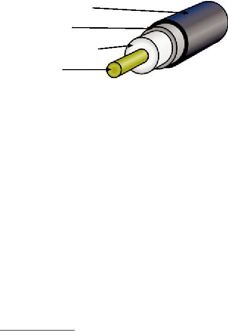
Coax
cables
have a core conductor
wire
surrounded by a non-conductive
material
called
dielectric,
or simply
insulation. The
dielectric is then surrounded
by
an
encompassing shielding which is
often made of braided wires.
The di-
electric
prevents an electrical connection
between the core and
the shielding.
Finally,
the coax is protected by an
outer casing which is
generally made
1.
Radio
Frequency. See chapter two
for discussion of electromagnetic
waves.
95
96
Chapter
4: Antennas & Transmission
Lines
from
a PVC material. The inner
conductor carries the RF
signal, and the
outer
shield prevents the RF
signal from radiating to the
atmosphere, and
also
prevents outside signals
from interfering with the
signal carried by the
core.
Another interesting fact is
that high frequency
electrical signal
always
travels
along the outer layer of a
conductor: the larger the
central conductor,
the
better signal will flow.
This is called the "skin
effect".
Outer
Jacket
Shield
Dielectric
Conductor
Figure
4.1: Coaxial cable with
jacket, shield, dielectric,
and core
conductor.
Even
though the coaxial
construction is good at containing
the signal on the
core
wire, there is some
resistance to the electrical flow:
as the signal travels
down
the core, it will fade
away. This fading is known
as attenuation, and
for
transmission
lines it is measured in decibels
per meter (dB/m). The
rate of
attenuation
is a function of the signal
frequency and the physical
construction
of
the cable itself. As the
signal frequency increases, so
does its attenuation.
Obviously,
we need to minimize the
cable attenuation as much as
possible
by
keeping the cable very
short and using high
quality cables.
Here
are some points to consider
when choosing a cable for
use with micro-
wave
devices:
1.
"The shorter the better!"
The first
rule when you install a
piece of cable is
to
try to keep it as short as
possible. The power loss is
not linear, so
doubling
the cable length means
that you are going to
lose much more
than
twice the power. In the
same way, reducing the
cable length by half
gives
you more than twice
the power at the antenna.
The best solution is
to
place the transmitter as
close as possible to the
antenna, even when
this
means placing it on a
tower.
2.
"The cheaper the worse!"
The second golden rule is
that any money
you
invest
in buying a good
quality cable is a
bargain. Cheap cables
are
intended
to be used at low frequencies,
such as VHF. Microwaves
re-
quire
the highest quality cables
available. All other options
are nothing
but
a dummy load2.
2.
A
dummy load is a device that
dissipates RF energy without
radiating it. Think of it as a
heat
sink
that works at radio
frequencies.
Chapter
4: Antennas & Transmission
Lines
97
3.
Always avoid RG-58. It is
intended for thin Ethernet
networking, CB or
VHF
radio, not for
microwave.
4.
Always avoid RG-213. It is
intended for CB and HF
radio. In this case
the
cable
diameter does not imply a
high quality, or low
attenuation.
5.
Whenever possible, use
Heliax
(also
called "Foam") cables for
connect-
ing
the transmitter to the
antenna. When Heliax is
unavailable, use the
best
rated LMR cable you
can find.
Heliax cables have a solid
or tubular
center
conductor with a corrugated
solid outer conductor to
enable them
to
flex.
Heliax can be built in two
ways, using either air or
foam as a di-
electric.
Air dielectric Heliax is the
most expensive and
guarantees the
minimum
loss, but it is very
difficult to
handle. Foam dielectric
Heliax is
slightly
more lossy, but is less
expensive and easier to
install. A special
procedure
is required when soldering
connectors in order to keep
the
foam
dielectric dry and
uncorrupted. LMR is a brand of
coax cable avail-
able
in various diameters that
works well at microwave
frequencies.
LMR-400
and LMR-600 are a commonly
used alternative to
Heliax.
6.
Whenever possible, use
cables that are pre-crimped
and tested in a
proper
lab. Installing connectors to
cable is a tricky business,
and is dif-
ficult to do
properly even with the
proper tools. Unless you
have access
to
equipment that can verify a
cable you make yourself
(such as a spec-
trum
analyzer and signal
generator, or time domain reflectometer),
trou-
bleshooting
a network that uses homemade
cable can be difficult.
7.
Don t
abuse
your transmission line.
Never step over a cable,
bend it too
much,
or try to unplug a connector by
pulling directly the cable.
All of
those
behaviors may change the
mechanical characteristic of the
cable
and
therefore its impedance,
short the inner conductor to
the shield, or
even
break the line. Those
problems are difficult to
track and recognize
and
can lead to unpredictable
behavior on the radio
link.
Waveguides
Above
2 GHz, the wavelength is
short enough to allow
practical, efficient
en-
ergy
transfer by different means. A
waveguide is a conducting tube
through
which
energy is transmitted in the
form of electromagnetic waves.
The tube
acts
as a boundary that confines
the waves in the enclosed
space. The
Faraday
cage effect prevents
electromagnetic effects from
being evident out-
side
the guide. The
electromagnetic fields
are propagated through
the
waveguide
by means of reflections
against its inner walls,
which are consid-
ered
perfect conductors. The
intensity of the fields is
greatest at the
center
along
the X dimension, and must
diminish to zero at the end
walls because
the
existence of any field
parallel to the walls at the
surface would cause
an
infinite
current to flow in a
perfect conductor. Waveguides, of
course, cannot
carry
RF in this fashion.
98
Chapter
4: Antennas & Transmission
Lines
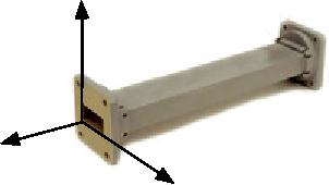
The
X, Y and Z dimensions of a rectangular
waveguide can be seen in
the
following
figure:
Y
Z
X
Figure
4.2: The X, Y, and Z
dimensions of a rectangular
waveguide.
There
are an infinite
number of ways in which the
electric and magnetic fields
can
arrange themselves in a waveguide
for frequencies above the
low cutoff
frequency.
Each of these field
configurations is
called a mode. The
modes
may
be separated into two
general groups. One group,
designated TM
(Transverse
Magnetic), has the magnetic
field
entirely transverse to the
di-
rection
of propagation, but has a
component of the electric field
in the direc-
tion
of propagation. The other
type, designated TE
(Transverse
Electric) has
the
electric field
entirely transverse, but has
a component of magnetic field
in
the
direction of propagation.
The
mode of propagation is identified by
the group letters followed
by two
subscript
numerals. For example, TE
10, TM 11, etc. The
number of possi-
ble
modes increases with the
frequency for a given size
of guide, and there
is
only one possible mode,
called the dominant
mode, for
the lowest fre-
quency
that can be transmitted. In a
rectangular guide, the
critical dimen-
sion
is X. This dimension must be
more than 0.5 at the
lowest frequency
to
be transmitted. In practice, the Y
dimension usually is made
about equal
to
0.5 X to avoid the
possibility of operation in other
than the dominant
mode.
Cross-sectional shapes other
than the rectangle can be
used, the
most
important being the circular
pipe. Much the same
considerations apply
as
in the rectangular case.
Wavelength dimensions for
rectangular and cir-
cular
guides are given in the
following table, where X is
the width of a rec-
tangular
guide and r is the radius of
a circular guide. All
figures apply to the
dominant
mode.

Chapter
4: Antennas & Transmission
Lines
99
Type
of guide
Rectangular
Circular
Cutoff
wavelength
2X
3.41r
Longest
wavelength
transmitted
with little
1.6X
3.2r
attenuation
Shortest
wavelength
before
next mode
1.1X
2.8r
becomes
possible
Energy
may be introduced into or
extracted from a waveguide by
means of
either
an electric or magnetic field.
The energy transfer
typically happens
through
a coaxial line. Two possible
methods for coupling to a
coaxial line
are
using the inner conductor of
the coaxial line, or through
a loop. A probe
which
is simply a short extension of
the inner conductor of the
coaxial line
can
be oriented so that it is parallel to
the electric lines of force.
A loop can
be
arranged so that it encloses
some of the magnetic lines
of force. The point
at
which maximum coupling is
obtained depends upon the
mode of propaga-
tion
in the guide or cavity.
Coupling is maximum when the
coupling device is
in
the most intense field.
If
a waveguide is left open at
one end, it will radiate
energy (that is, it can
be
used
as an antenna rather than as a
transmission line). This
radiation can be
enhanced
by flaring
the waveguide to form a
pyramidal horn antenna. We
will
see
an example of a practical waveguide
antenna for WiFi later in
this chap-
ter.
Cable
Type
Core
Dielectric
Shield
Jacket
RG-58
0.9
mm
2.95
mm
3.8
mm
4.95
mm
RG-213
2.26
mm
7.24
mm
8.64
mm
10.29
mm
LMR-400
2.74
mm
7.24
mm
8.13
mm
10.29
mm
3/8"
LDF
3.1
mm
8.12
mm
9.7
mm
11
mm
Here
is a table contrasting the
sizes of various common
transmission lines.
Choose
the best cable you
can afford with the
lowest possible attenuation
at
the
frequency you intend to use
for your wireless
link.
100
Chapter
4: Antennas & Transmission
Lines
Connectors
and adapters
Connectors
allow a cable to be connected to
another cable or to a
compo-
nent
of the RF chain. There are a
wide variety of fittings
and connectors de-
signed
to go with various sizes and
types of coaxial lines. We
will describe
some
of the most popular
ones.
BNC
connectors were
developed in the late 40s.
BNC stands for
Bayonet
Neill
Concelman, named after the
men who invented it:
Paul Neill and
Carl
Concelman.
The BNC product line is a
miniature quick connect /
disconnect
connector.
It features two bayonet lugs
on the female connector, and
mating
is
achieved with only a quarter
turn of the coupling nut.
BNC's are ideally
suited
for cable termination for
miniature to subminiature coaxial
cable (RG-
58
to RG-179, RG-316, etc.)
They have acceptable
performance up to few
GHz.
They are most commonly
found on test equipment and
10base2 coax-
ial
Ethernet cables.
TNC
connectors were
also invented by Neill and
Concelman, and are a
threaded
variation of the BNC. Due to
the better interconnect
provided by
the
threaded connector, TNC
connectors work well through
about 12 GHz.
TNC
stands for Threaded Neill
Concelman.
Type
N (again
for Neill, although
sometimes attributed to "Navy")
connectors
were
originally developed during
the Second World War.
They are usable up
to
18 Ghz, and very commonly
used for microwave
applications. They
are
available
for almost all types of
cable. Both the plug /
cable and plug /
socket
joints
are waterproof, providing an
effective cable
clamp.
SMA
is an acronym
for SubMiniature version A,
and was developed in
the
60s.
SMA connectors are
precision, subminiature units
that provide
excellent
electrical
performance up to 18 GHz. These
high-performance connectors
are
compact in size and
mechanically have outstanding
durability.
The
SMB
name
derives from SubMiniature B,
and it is the second
subminia-
ture
design. The SMB is a smaller
version of the SMA with
snap-on coupling.
It
provides broadband capability
through 4 GHz with a snap-on
connector
design.
MCX
connectors
were introduced in the 80s.
While the MCX uses
identical
inner
contact and insulator
dimensions as the SMB, the
outer diameter of the
plug
is 30% smaller than the
SMB. This series provides
designers with op-
tions
where weight and physical
space are limited. MCX
provides broadband
capability
though 6 GHz with a snap-on
connector design.
Chapter
4: Antennas & Transmission
Lines
101
In
addition to these standard
connectors, most WiFi
devices use a variety
of
proprietary
connectors. Often, these
are simply standard
microwave con-
nectors
with the center conductor
parts reversed, or the
thread cut in the
op-
posite
direction. These parts are
often integrated into a
microwave system
using
a short jumper called a
pigtail
that
converts the non-standard
connec-
tor
into something more robust
and commonly available.
Some of these
connectors
include:
RP-TNC. This is a
TNC connector with the
genders reversed. These
are
most
commonly found on Linksys
equipment, such as the
WRT54G.
U.FL
(also
known as MHF). The
U.FL is a patented connector
made by Hi-
rose,
while the MHF is a
mechanically equivalent connector.
This is possibly
the
smallest microwave connector
currently in wide use. The
U.FL / MHF is
typically
used to connect a mini-PCI
radio card to an antenna or
larger con-
nector
(such as an N or TNC).
The
MMCX
series,
which is also called a
MicroMate, is one of the
smallest
RF
connector line and was
developed in the 90s. MMCX
is a micro-miniature
connector
series with a lock-snap
mechanism allowing for 360
degrees rota-
tion
enabling flexibility.
MMCX connectors are commonly
found on PCMCIA
radio
cards, such as those
manufactured by Senao and
Cisco.
MC-Card
connectors
are even smaller and
more fragile than MMCX.
They
have
a split outer connector that
breaks easily after just a
few interconnects.
These
are commonly found on Lucent
/ Orinoco / Avaya
equipment.
Adapters,
which are also called
coaxial adapters, are short,
two-sided connec-
tors
which are used to join
two cables or components
which cannot be con-
nected
directly. Adapters can be
used to interconnect devices or
cables with
different
types. For example, an
adapter can be used to
connect an SMA con-
nector
to a BNC. Adapters may also
be used to fit together
connectors of the
same
type, but which cannot be
directly joined because of
their gender.
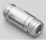
Figure
4.3: An N female barrel
adapter.
For
example a very useful
adapter is the one which
enables to join two
Type
N
connectors, having socket
(female) connectors on both
sides.
102
Chapter
4: Antennas & Transmission
Lines
Choosing
the proper connector
1.
"The gender question."
Virtually all connectors
have a well defined
gen-
der
consisting of either a pin
(the "male" end) or a socket
(the "female"
end).
Usually cables have male
connectors on both ends,
while RF de-
vices
(i.e. transmitters and
antennas) have female
connectors. Devices
such
as directional couplers and
line-through measuring devices
may
have
both male and female
connectors. Be sure that
every male con-
nector
in your system mates with a
female connector.
2.
"Less is best!" Try to
minimize the number of
connectors and adapters
in
the
RF chain. Each connector
introduces some additional
loss (up to a
few
dB for each connection,
depending on the
connector!)
3.
"Buy, don t
build!" As
mentioned earlier, buy
cables that are already
ter-
minated
with the connectors you
need whenever possible.
Soldering
connectors
is not an easy task, and to
do this job properly is
almost im-
possible
for small connectors as U.FL
and MMCX. Even
terminating
"Foam"
cables is not an easy
task.
4.
Don t
use
BNC for 2.4 GHz or higher.
Use N type connectors (or
SMA,
SMB,
TNC, etc.)
5.
Microwave connectors are
precision-made parts, and
can be easily
damaged
by mistreatment. As a general rule,
you should rotate the
outer
sleeve
to tighten the connector,
leaving the rest of the
connector (and
cable)
stationary. If other parts of
the connector are twisted
while tighten-
ing
or loosening, damage can
easily occur.
6.
Never step over connectors,
or drop connectors on the floor
when dis-
connecting
cables (this happens more
often than what you
may imagine,
especially
when working on a mast over
a roof).
7.
Never use tools like
pliers to tighten connectors.
Always use your
hands.
When
working outside, remember
that metals expand at high
tempera-
tures
and reduce their size at
low temperatures: a very
tightened connec-
tor
in the summer can bind or
even break in winter.
Antennas
& radiation patterns
Antennas
are a very important
component of communication systems.
By
definition,
an antenna is a device used to
transform an RF signal traveling
on
a
conductor into an electromagnetic
wave in free space. Antennas
demon-
strate
a property known as reciprocity, which
means that an antenna
will
maintain
the same characteristics
regardless if whether it is transmitting
or
receiving.
Most antennas are
resonant devices, which
operate efficiently
over
a relatively narrow frequency
band. An antenna must be
tuned to the
same
frequency band of the radio
system to which it is connected,
otherwise
Chapter
4: Antennas & Transmission
Lines
103
the
reception and the
transmission will be impaired.
When a signal is fed
into
an
antenna, the antenna will
emit radiation distributed in
space in a certain
way.
A graphical representation of the
relative distribution of the
radiated
power
in space is called a radiation
pattern.
Antenna
term glossary
Before
we talk about specific antennas,
there are a few common
terms that
must
be defined
and explained:
Input
Impedance
For
an efficient
transfer of energy, the
impedance
of the
radio, antenna, and
transmission
cable connecting them must
be the same. Transceivers
and
their
transmission lines are
typically designed for 50
impedance. If the
an-
tenna
has an impedance different
than 50 ,
then
there is a mismatch and
an
impedance
matching circuit is required.
When any of these components
are
mismatched,
transmission efficiency
suffers.
Return
loss
Return
loss is another
way of expressing mismatch. It is a
logarithmic ratio
measured
in dB that compares the
power reflected by
the antenna to the
power
that is fed into the
antenna from the
transmission line. The
relation-
ship
between SWR and return
loss is the
following:
SWR
Return
Loss (in dB) = 20log10
SWR-1
While
some energy will always be
reflected
back into the system, a
high re-
turn
loss will yield unacceptable
antenna performance.
Bandwidth
The
bandwidth
of an antenna
refers to the range of
frequencies over
which
the
antenna can operate
correctly. The antenna's
bandwidth is the number
of
Hz
for which the antenna
will exhibit an SWR less
than 2:1.
The
bandwidth can also be
described in terms of percentage of
the center
frequency
of the band.
FH -
FL
Bandwidth
= 100
FC
104
Chapter
4: Antennas & Transmission
Lines
...where
FH is
the highest frequency in the
band, FL
is the
lowest frequency in
the
band, and FC is the center frequency in
the band.
In
this way, bandwidth is constant relative
to frequency. If bandwidth was
ex-
pressed
in absolute units of frequency, it would be
different depending upon the
center
frequency. Different types of antennas have
different bandwidth limitations.
Directivity
and Gain
Directivity
is the
ability of an antenna to focus
energy in a particular
direction
when
transmitting, or to receive energy
from a particular direction
when re-
ceiving.
If a wireless link uses fixed
locations for both ends, it
is possible to
use
antenna directivity to concentrate
the radiation beam in the
wanted direc-
tion.
In a mobile application where
the transceiver is not fixed, it
may be im-
possible
to predict where the
transceiver will be, and so
the antenna should
ideally
radiate as well as possible in
all directions. An omnidirectional
an-
tenna
is used in these
applications.
Gain
is not a
quantity which can be defined
in terms of a physical
quantity
such
as the Watt or the Ohm,
but it is a dimensionless ratio.
Gain is given in
reference
to a standard antenna. The
two most common reference
antennas
are
the isotropic
antenna and
the resonant
half-wave dipole
antenna.
The
isotropic antenna radiates
equally well in all
directions. Real
isotropic
antennas
do not exist, but they
provide useful and simple
theoretical antenna
patterns
with which to compare real
antennas. Any real antenna
will radiate
more
energy in some directions
than in others. Since
antennas cannot
create
energy,
the total power radiated is
the same as an isotropic
antenna. Any
additional
energy radiated in the
directions it favors is offset by
equally less
energy
radiated in all other
directions.
The
gain of an antenna in a given
direction is the amount of
energy radiated
in
that direction compared to
the energy an isotropic
antenna would radiate
in
the
same direction when driven
with the same input
power. Usually we are
only
interested in the maximum
gain, which is the gain in
the direction in
which
the antenna is radiating
most of the power. An
antenna gain of 3 dB
compared
to an isotropic antenna would be
written as 3
dBi. The
resonant
half-wave
dipole can be a useful
standard for comparing to
other antennas at
one
frequency or over a very
narrow band of frequencies. To
compare the
dipole
to an antenna over a range of
frequencies requires a number of
di-
poles
of different lengths. An antenna
gain of 3 dB compared to a dipole
an-
tenna
would be written as 3
dBd.
The
method of measuring gain by
comparing the antenna under
test against a
known
standard antenna, which has
a calibrated gain, is technically
known as
a
gain
transfer technique.
Another method for measuring
gain is the 3 anten-
Chapter
4: Antennas & Transmission
Lines
105
nas
method, where the
transmitted and received
power at the antenna
termi-
nals
is measured between three
arbitrary antennas at a known
fixed distance.
Radiation
Pattern
The
radiation
pattern or
antenna
pattern describes
the relative strength
of
the
radiated field in
various directions from the
antenna, at a constant
dis-
tance.
The radiation pattern is a
reception pattern as well,
since it also de-
scribes
the receiving properties of
the antenna. The radiation
pattern is three-
dimensional,
but usually the measured
radiation patterns are a
two-
dimensional
slice of the three-dimensional
pattern, in the horizontal or
verti-
cal
planes. These pattern
measurements are presented in
either a rectangu-
lar
or a
polar
format.
The following figure
shows a rectangular plot
presenta-
tion
of a typical ten-element Yagi.
The detail is good but it is
difficult to
visual-
ize
the antenna behavior in
different directions.
dB
-5
-10
-15
-20
-25
-30
-35
-40
-45
-50
-180°
-140°
-100°
-60°
-20°
20°
60°
100°
140°
180°
Figure
4.4: A rectangular plot of a
yagi radiation
pattern.
Polar
coordinate systems are used
almost universally. In the
polar-coordinate
graph,
points are located by
projection along a rotating
axis (radius) to an
intersection
with one of several
concentric circles. The
following is a polar
plot
of the same 10 element Yagi
antenna.
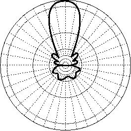
Polar
coordinate systems may be
divided generally in two
classes: linear
and
logarithmic. In the
linear coordinate system,
the concentric circles
are
equally
spaced, and are graduated.
Such a grid may be used to
prepare a
linear
plot of the power contained
in the signal. For ease of
comparison, the
equally
spaced concentric circles
may be replaced with
appropriately placed
circles
representing the decibel
response, referenced to 0 dB at the
outer
edge
of the plot. In this kind of
plot the minor lobes
are suppressed. Lobes
with
peaks more than 15 dB or so
below the main lobe
disappear because of
their
small size. This grid
enhances plots in which the
antenna has a high
directivity
and small minor lobes.
The voltage of the signal,
rather than the
power,
can also be plotted on a
linear coordinate system. In
this case, too,
106
Chapter
4: Antennas & Transmission
Lines
the
directivity is enhanced and
the minor lobes suppressed,
but not in the
same
degree as in the linear
power grid.
0°
270°
90°
180°
Figure
4.5: A linear polar plot of
the same yagi.
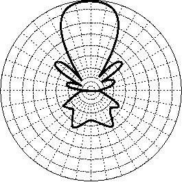
In
the logarithmic polar
coordinate system the
concentric grid lines
are
spaced
periodically according to the
logarithm of the voltage in
the signal.
Different
values may be used for
the logarithmic constant of
periodicity, and
this
choice will have an effect
on the appearance of the
plotted patterns.
Generally
the 0 dB reference for the
outer edge of the chart is
used. With this
type
of grid, lobes that are 30
or 40 dB below the main lobe
are still distin-
guishable.
The spacing between points
at 0 dB and at -3 dB is greater
than
the
spacing between -20 dB and
-23 dB, which is greater
than the spacing
between
-50 dB and -53 dB.
The spacing thus correspond
to the relative sig-
nificance
of such changes in antenna
performance.
A
modified logarithmic scale
emphasizes the shape of the
major beam while
compressing
very low-level (>30 dB)
sidelobes towards the center of
the pattern.
This
is shown in Figure
4.6.
There
are two kinds of radiation
pattern: absolute
and
relative.
Absolute
radiation
patterns are presented in
absolute units of field
strength or power.
Relative
radiation patterns are
referenced in relative units of
field
strength or
power.
Most radiation pattern
measurements are relative to
the isotropic an-
tenna,
and the gain transfer
method is then used to
establish the
absolute
gain
of the antenna.
Chapter
4: Antennas & Transmission
Lines
107
0°
270°
90°
180°
Figure
4.6: The logarithmic polar
plot
The
radiation pattern in the
region close to the antenna
is not the same as
the
pattern at large distances.
The term near-field
refers to the field
pattern
that
exists close to the antenna,
while the term
far-field
refers to the field
pat-
tern
at large distances. The
far-field is
also called the radiation
field,
and is
what
is most commonly of interest.
Ordinarily, it is the radiated
power that is
of
interest, and so antenna
patterns are usually
measured in the far-field
re-
gion.
For pattern measurement it is
important to choose a distance
suffi-
ciently
large to be in the far-field,
well out of the
near-field.
The minimum
permissible
distance depends on the
dimensions of the antenna in
relation to
the
wavelength. The accepted
formula for this distance
is:
2d2
rmin =
w
here
rmin is the minimum distance
from the antenna, d is the
largest dimen-
sion
of the antenna, and is the
wavelength.
Beamwidth
An
antenna's beamwidth
is usually
understood to mean the
half-power
beamwidth.
The peak radiation intensity
is found, and then the
points on ei-
ther
side of the peak which
represent half the power of
the peak intensity
are
located.
The angular distance between
the half power points is
defined
as
the
beamwidth. Half the power
expressed in decibels is -3dB, so
the half
power
beamwidth is sometimes referred to as
the 3dB beamwidth. Both
hori-
zontal
and vertical beamwidth are
usually considered.
108
Chapter
4: Antennas & Transmission
Lines
Assuming
that most of the radiated
power is not divided into
sidelobes, then
the
directive gain is inversely
proportional to the beamwidth: as
the beam-
width
decreases, the directive
gain increases.
Sidelobes
No
antenna is able to radiate
all the energy in one
preferred direction.
Some
is
inevitably radiated in other
directions. These smaller
peaks are referred to
as
sidelobes, commonly
specified in dB down
from the main
lobe.
Nulls
In
an antenna radiation pattern, a
null
is a zone in
which the effective
radi-
ated
power is at a minimum. A null
often has a narrow
directivity angle
com-
pared
to that of the main beam.
Thus, the null is useful
for several purposes,
such
as suppression of interfering signals in
a given direction.
Polarization
Polarization
is defined as
the orientation of the
electric field of an
electro-
magnetic
wave. Polarization is in general
described by an ellipse. Two
spe-
cial
cases of elliptical polarization
are linear
polarization and
circular
po-
larization. The
initial polarization of a radio
wave is determined by the
an-
tenna.
direction
of propagation
electric
field
magnetic
field
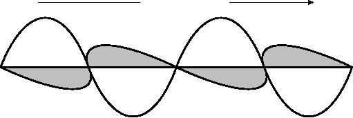
Figure
4.7: The electrical wave is
perpendicular to magnetic wave,
both of which are
perpendicular
to the direction of
propagation.
With
linear polarization, the
electric field vector stays
in the same plane
all
the
time. The electric field
may leave the antenna in a
vertical orientation, a
horizontal
orientation, or at some angle
between the two.
Vertically
polar-
ized
radiation is
somewhat less affected by
reflections over the
transmis-
sion
path. Omnidirectional antennas
always have vertical
polarization. With
horizontal
polarization, such
reflections cause variations in
received sig-
nal
strength. Horizontal antennas
are less likely to pick up
man-made inter-
ference,
which ordinarily is vertically
polarized.
Chapter
4: Antennas & Transmission
Lines
109
In
circular polarization the
electric field
vector appears to be rotating
with
circular
motion about the direction
of propagation, making one
full turn for
each
RF cycle. This rotation may
be right-hand or left-hand. Choice of
polari-
zation
is one of the design choices
available to the RF system
designer.
Polarization
Mismatch
In
order to transfer maximum
power between a transmit and
a receive an-
tenna,
both antennas must have
the same spatial
orientation, the same
po-
larization
sense, and the same
axial ratio.
When
the antennas are not
aligned or do not have the
same polarization,
there
will be a reduction in power
transfer between the two
antennas. This
reduction
in power transfer will
reduce the overall system
efficiency
and per-
formance.
When
the transmit and receive
antennas are both linearly
polarized, physical
antenna
misalignment will result in a
polarization mismatch loss,
which can
be
determined using the
following formula:
Loss
(dB) = 20 log (cos
)
...where
is the difference in alignment
angle between the two
antennas. For
15°
the loss is approximately
0.3dB, for 30° we lose
1.25dB, for 45° we
lose
3dB
and for 90° we have an
infinite
loss.
In
short, the greater the
mismatch in polarization between a
transmitting and
receiving
antenna, the greater the
apparent loss. In the
real world, a 90°
mismatch
in polarization is quite large
but not infinite.
Some antennas, such
as
yagis or can antennas, can
be simply rotated 90° to
match the
polarization
of
the other end of the
link. You can use
the polarization effect to
your ad-
vantage
on a point-to-point link. Use a
monitoring tool to observe
interfer-
ence
from adjacent networks, and
rotate one antenna until
you see the
low-
est
received signal. Then bring
your link online and
orient the other end
to
match
polarization. This technique
can sometimes be used to
build stable
links,
even in noisy radio
environments.
Front-to-back
ratio
It
is often useful to compare
the front-to-back
ratio of directional
antennas.
This
is the ratio of the maximum
directivity of an antenna to its
directivity in
the
opposite direction. For
example, when the radiation
pattern is plotted on
a
relative dB scale, the
front-to-back ratio is the
difference in dB between
the
level
of the maximum radiation in
the forward direction and
the level of radia-
tion
at 180 degrees.
110
Chapter
4: Antennas & Transmission
Lines
This
number is meaningless for an
omnidirectional antenna, but it
gives you
an
idea of the amount of power
directed forward on a very
directional an-
tenna.
Types
of Antennas
A
classification of
antennas can be based
on:
·
Frequency
and size. Antennas
used for HF are different
from antennas
used
for VHF, which in turn
are different from antennas
for microwave. The
wavelength
is different at different frequencies, so
the antennas must be
different
in size to radiate signals at
the correct wavelength. We
are par-
ticularly
interested in antennas working in
the microwave range,
especially
in
the 2.4 GHz and 5
GHz frequencies. At 2.4 GHz
the wavelength is
12.5
cm,
while at 5 GHz it is 6
cm.
·
Directivity.
Antennas
can be omnidirectional, sectorial or
directive. Omni-
directional
antennas radiate
roughly the same pattern
all around the
an-
tenna
in a complete 360° pattern.
The most popular types of
omnidirec-
tional
antennas are the
dipole
and
the ground
plane.
Sectorial
antennas
radiate
primarily in a specific area.
The beam can be as wide as
180 de-
grees,
or as narrow as 60 degrees.
Directional
or
directive
antennas are
antennas
in which the beamwidth is
much narrower than in
sectorial an-
tennas.
They have the highest
gain and are therefore
used for long
dis-
tance
links. Types of directive
antennas are the Yagi,
the biquad, the
horn,
the
helicoidal, the patch
antenna, the parabolic dish,
and many others.
·
Physical
construction. Antennas
can be constructed in many
different
ways,
ranging from simple wires,
to parabolic dishes, to coffee
cans.
When
considering antennas suitable
for 2.4 GHz WLAN
use, another classi-
fication
can be used:
·
Application.
Access points tend to make
point-to-multipoint networks,
while
remote links are
point-to-point. Each of these
suggest different
types
of
antennas for their purpose.
Nodes that are used
for multipoint access
will
likely use omni antennas
which radiate equally in all
directions, or sec-
torial
antennas which focus into a
small area. In the
point-to-point case,
antennas
are used to connect two
single locations together.
Directive an-
tennas
are the primary choice
for this application.
A
brief list of common type of
antennas for the 2.4
GHz frequency is pre-
sented
now, with a short
description and basic
information about their
char-
acteristics.
Chapter
4: Antennas & Transmission
Lines
111
1/4
wavelength ground plane
The
1/4 wavelength
ground plane antenna is very
simple in its
construction
and
is useful for communications
when size, cost and
ease of construction
are
important. This antenna is
designed to transmit a vertically
polarized sig-
nal.
It consists of a 1/4 wave
element as half-dipole and
three or four 1/4
wavelength
ground elements bent 30 to 45
degrees down. This set of
ele-
ments,
called radials, is known as a
ground plane.
Figure
4.8: Quarter wavelength
ground plane
antenna.
This
is a simple and effective
antenna that can capture a
signal equally from
all
directions. To increase the
gain, the signal can be
flattened
out to take
away
focus from directly above
and below, and providing
more focus on the
horizon.
The vertical beamwidth
represents the degree of flatness
in the fo-
cus.
This is useful in a Point-to-Multipoint
situation, if all the other
antennas
are
also at the same height.
The gain of this antenna is
in the order of 2 - 4
dBi.
Yagi
antenna
A
basic Yagi consists of a
certain number of straight
elements, each
measur-
ing
approximately half wavelength.
The driven or active element
of a Yagi is
the
equivalent of a center-fed, half-wave
dipole antenna. Parallel to
the
driven
element, and approximately
0.2 to 0.5 wavelength on
either side of it,
are
straight rods or wires
called reflectors
and directors, or simply
passive
elements.
A reflector
is placed behind the driven
element and is
slightly
longer
than half wavelength; a
director is placed in front of
the driven element
and
is slightly shorter than
half wavelength. A typical
Yagi has one reflector
and
one or more directors. The
antenna propagates electromagnetic
field
energy
in the direction running
from the driven element
toward the directors,
and
is most sensitive to incoming
electromagnetic field
energy in this same
direction.
The more directors a Yagi
has, the greater the
gain. As more direc-
112
Chapter
4: Antennas & Transmission
Lines
tors
are added to a Yagi, it
therefore becomes longer.
Following is the
photo
of
a Yagi antenna with 6
directors and one reflector.
Figure
4.9: A Yagi
antenna.
Yagi
antennas are used primarily
for Point-to-Point links,
have a gain from 10
to
20 dBi and a horizontal
beamwidth of 10 to 20 degrees.
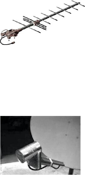
Horn
The
horn antenna derives its
name from the characteristic
flared appear-
ance.
The flared portion can be
square, rectangular, cylindrical or
conical.
The
direction of maximum radiation
corresponds with the axis of
the horn. It
is
easily fed with a waveguide,
but can be fed with a
coaxial cable and a
proper
transition.
Figure
4.10: Feed horn made
from a food can.
Horn
antennas are commonly used
as the active element in a
dish antenna.
The
horn is pointed toward the
center of the dish reflector.
The use of a horn,
rather
than a dipole antenna or any
other type of antenna, at
the focal point
of
the dish minimizes loss of
energy around the edges of
the dish reflector.
At
2.4
GHz, a simple horn antenna
made with a tin can
has a gain in the
order
of
10 - 15 dBi.
Chapter
4: Antennas & Transmission
Lines
113
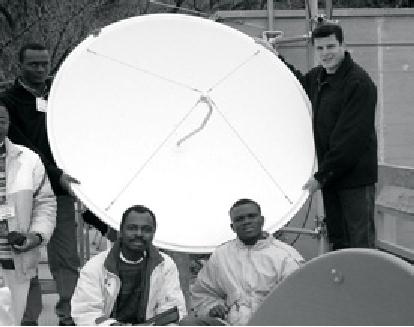
Parabolic
Dish
Antennas
based on parabolic reflectors
are the most common
type of directive
antennas
when a high gain is
required. The main advantage
is that they can be
made
to have gain and directivity
as large as required. The
main disadvantage
is
that big dishes are
difficult to mount and are
likely to have a large
windage.
Figure
4.11: A solid dish
antenna.
Dishes
up to one meter are usually
made from solid material.
Aluminum is
frequently
used for its weight
advantage, its durability
and good electrical
characteristics.
Windage increases rapidly
with dish size and
soon becomes
a
severe problem. Dishes which
have a reflecting
surface that uses an
open
mesh
are frequently used. These
have a poorer front-to-back
ratio, but are
safer
to use and easier to build.
Copper, aluminum, brass,
galvanized steel
and
iron are suitable mesh
materials.
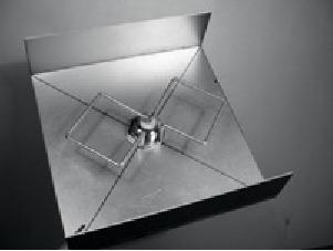
BiQuad
The
BiQuad antenna is simple to
build and offers good
directivity and gain
for
Point-to-Point
communications. It consists of a two
squares of the same size
of
1/4
wavelength as a radiating element
and of a metallic plate or
grid as reflec-
tor.
This antenna has a beamwidth
of about 70 degrees and a
gain in the order
of
10-12 dBi. It can be used as
stand-alone antenna or as feeder
for a Para-
bolic
Dish. The polarization is
such that looking at the
antenna from the front,
if
the
squares are placed side by
side the polarization is
vertical.
114
Chapter
4: Antennas & Transmission
Lines
Figure
4.12: The BiQuad.
Other
Antennas
Many
other types of antennas
exist and new ones
are created following
the
advances
in technology.
·
Sector or Sectorial antennas:
they are widely used in
cellular telephony
infrastructure
and are usually built
adding a reflective
plate to one or more
phased
dipoles. Their horizontal
beamwidth can be as wide as
180 de-
grees,
or as narrow as 60 degrees, while
the vertical is usually much
nar-
rower.
Composite antennas can be
built with many Sectors to
cover a
wider
horizontal range (multisectorial
antenna).
·
Panel or Patch antennas:
they are solid flat panels
used for indoor
cover-
age,
with a gain up to 20
dB.
Reflector
theor y
The
basic property of a perfect
parabolic reflector is
that it converts a
spheri-
cal
wave irradiating from a
point source placed at the
focus into a plane
wave.
Conversely, all the energy
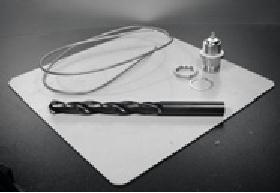
received by the dish from a
distant source is
reflected
to a single point at the
focus of the dish. The
position of the
focus,
or
focal length, is given
by:
D2
f=
16
c
...where
D is the dish diameter and c
is the depth of the parabola
at its center.
Chapter
4: Antennas & Transmission
Lines
115
The
size of the dish is the
most important factor since
it determines the
maximum
gain that can be achieved at
the given frequency and
the resulting
beamwidth.
The gain and beamwidth
obtained are given
by:
D)2
(
Gain
=
n
2
B
70
eamwidth
=
D
...where
D is the dish diameter and n
is the efficiency.
The efficiency is
de-
termined
mainly by the effectiveness of
illumination of the dish by
the feed,
but
also by other factors. Each
time the diameter of a dish
is doubled, the
gain
is four times, or 6 dB,
greater. If both stations
double the size of
their
dishes,
signal strength can be
increased of 12 dB, a very
substantial gain. An
efficiency
of 50% can be assumed when
hand-building the
antenna.
The
ratio f / D (focal length/diameter of
the dish) is the fundamental
factor
governing
the design of the feed
for a dish. The ratio is
directly related to
the
beamwidth
of the feed necessary to
illuminate the dish
effectively. Two
dishes
of the same diameter but
different focal lengths
require different de-
sign
of feed if both are to be
illuminated efficiently.
The value of 0.25
corre-
sponds
to the common focal-plane
dish in which the focus is
in the same
plane
as the rim of the
dish.
Amplifiers
As
mentioned earlier, antennas do
not actually create power.
They simply
direct
all available power into a
particular pattern. By using a
power
ampli-
fier, you
can use DC power to augment
your available signal. An
amplifier
connects
between the radio
transmitter and the antenna,
and has an addi-
tional
lead that connects to a
power source. Amplifiers
are available that
work
at 2.4 GHz,
and can add several
Watts of power to your
transmission.
These
devices sense when an
attached radio is transmitting,
and quickly
power
up and amplify the signal.
They then switch off
again when transmis-
sion
ends. When receiving, they
also add amplification to
the signal before
sending
it to the radio.
Unfortunately,
simply adding amplifiers
will not magically solve
all of your
networking
problems. We do not discuss
power amplifiers at
length in this
book
because there are a number
of significant
drawbacks to using
them:
·
They
are expensive. Amplifiers
must work at relatively wide
bandwidths at
2.4
GHz,
and must switch quickly
enough to work for Wi-Fi
applications.
116
Chapter
4: Antennas & Transmission
Lines
These
amplifiers do
exist, but they tend to
cost several hundred dollars
per
unit.
·
You
will need at least two.
Whereas antennas provide
reciprocal gain
that
benefits both
sides of a connection, amplifiers
work best at
amplifying
a
transmitted signal. If you
only add an amplifier to one
end of a link with
insufficient
antenna gain, it will likely
be able to be heard but will
not be
able
to hear the other
end.
·
They
provide no additional directionality.
Adding
antenna gain provides
both
gain and directionality
benefits to both
ends of the link. They
not only
improve
the available amount of
signal, but tend to reject
noise from other
directions.
Amplifiers
blindly amplify both desired
and interfering
signals,
and
can make interference
problems worse.
·
Amplifiers
generate noise for other users of the
band. By
increasing
your
output power, you are
creating a louder source of
noise for other
us-
ers
of the unlicensed band. This
may not be much of an issue
today in
rural
areas, but it can cause
big problems in populated
areas. Conversely,
adding
antenna gain will improve
your link and can
actually decrease the
noise
level for your
neighbors.
·
Using
amplifiers
probably isn t
legal.
Every
country imposes power
lim-
its
on use of unlicensed spectrum.
Adding an antenna to a highly
amplified
signal
will likely cause the
link to exceed legal
limits.
Using
amplifiers is
often compared to the
inconsiderate neighbor who
wants
to
listen to the radio outside
their home, and so turns it
up to full volume.
They
might even "improve"
reception by pointing their
speakers out the
win-
dow.
While they may now be
able to hear the radio, so
must everyone else
on
the block. This approach
may scale to exactly one
user, but what
hap-
pens
when the neighbors decide to
do the same thing with
their radios? Us-
ing
amplifiers
for a wireless link causes
roughly the same effect at
2.4 GHz.
Your
link may "work better"
for the moment, but
you will have problems
when
other
users of the band decide to
use amplifiers of
their own.
By
using higher gain antennas
rather than amplifiers,
you avoid all of
these
problems.
Antennas cost far less
than amps, and can
improve a link simply
by
changing the antenna on one
end. Using more sensitive
radios and good
quality
cable also helps
significantly on
long distance shots.
These tech-
niques
are unlikely to cause
problems for other users of
the band, and so we
recommend
pursuing them before adding
amplifiers.
Practical
antenna designs
The
cost of 2.4 GHz antennas
has fallen dramatically
since the introduction
of
802.11b.
Innovative designs use
simpler parts and fewer
materials to achieve
Chapter
4: Antennas & Transmission
Lines
117
impressive
gain with relatively little
machining. Unfortunately,
availability of
good
antennas is still limited in
many areas of the world,
and importing them
can
be prohibitively expensive. While
actually designing an antenna
can be a
complex
and error-prone process, constructing
antennas from locally
available
components
is very straightforward, and
can be a lot of fun. We
present four
practical
antenna designs that can be
built for very little
money.
USB
dongle as dish feed
Possibly
the simplest antenna design
is the use of a parabola to
direct the
output
of a USB wireless device
(known in networking circles as a
USB
dongle). By
placing the internal dipole
antenna present in USB
wireless
dongles
at the focus of a parabolic
dish, you can provide
significant
gain
without
the need to solder or even
open the wireless device
itself. Many
kinds
of parabolic dishes will
work, including satellite
dishes, television
an-
tennas,
and even metal cookware
(such as a wok, round lid,
or strainer). As
a
bonus, inexpensive and
lossless USB cable is then
used to feed the
an-
tenna,
eliminating the need for
expensive coaxial cable or
Heliax.
To
build a USB dongle
parabolic, you will need to
find the orientation and
loca-
tion
of the dipole inside the
dongle. Most devices orient
the dipole to be paral-
lel
with the short edge of
the dongle, but some
will mount the dipole
perpen-
dicular
to the short edge. You
can either open the
dongle and look for
yourself,
or
simply try the dongle in
both positions to see which
provides more gain.
To
test the antenna, point it
at an access point several
meters away, and con-
nect
the USB dongle to a laptop.
Using the laptop s
client
driver or a tool such
as
Netstumbler (see Chapter
6),
observe the received signal
strength of the
access
point. Now, slowly move
the dongle in relation to
the parabolic while
watching
the signal strength meter.
You should see a significant
improvement
in
gain (20 dB or more) when
you find the proper
position. The proper
position
will
vary depending on the shape
of the parabola and the
construction of the
USB
dongle. Try various
positions while watching
your signal strength
meter
until
you find the
optimum location.
Once
the best location is found,
securely fix the
dongle in place. You
will
need
to waterproof the dongle and
cable if the antenna is used
outdoors.
Use
a silicone compound or a piece of
PVC tubing to seal the
electronics
against
the weather. Many USB-fed
parabolic designs and ideas
are docu-
mented
online at http://www.usbwifi.orcon.net.nz/
.
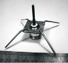
Collinear
omni
This
antenna is very simple to
build, requiring just a
piece of wire, an N
socket
and a square metallic plate.
It can be used for indoor or
outdoor point-
to-multipoint
short distance coverage. The
plate has a hole drilled in
the mid-
118
Chapter
4: Antennas & Transmission
Lines
dle
to accommodate an N type chassis
socket that is screwed into
place. The
wire
is soldered to the center
pin of the N socket and
has coils to separate
the
active phased elements. Two
versions of the antenna are
possible: one
with
two phased elements and
two coils and another
with four phased
ele-
ments
and four coils. For
the short antenna the
gain will be around 5 dBi,
while
the long one with
four elements will have 7 to
9 dBi of gain. We are
go-
ing
to describe how to build the
long antenna only.
Parts
list and tools
required
·
One screw-on N-type female
connector
·
50 cm of copper or brass wire of 2 mm of
diameter
·
10x10 cm or greater square
metallic plate
Figure
4.13: 10 cm x 10 cm aluminum
plate.
·
Ruler
·
Pliers
·
File
·
Soldering iron and
solder
·
Drill with a set of bits
for metal (including a 1.5
cm diameter bit)
·
A piece of pipe or a drill
bit with a diameter of 1
cm
·
Vice or clamp
·
Hammer
·
Spanner or monkey
wrench
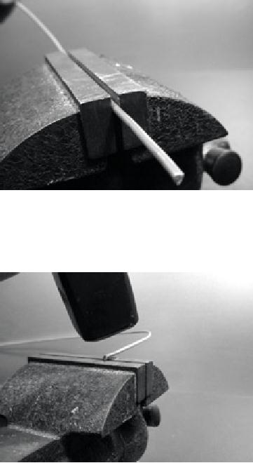
Construction
1.
Straighten the wire using
the vice.
Chapter
4: Antennas & Transmission
Lines
119
Figure
4.14: Make the wire as
straight as you
can.
2.
With a marker, draw a line
at 2.5 cm starting from one
end of the wire.
On
this line, bend the
wire at 90 degrees with the
help of the vice and
of
the
hammer.
Figure
4.15: Gently tap the
wire to make a sharp
bend.
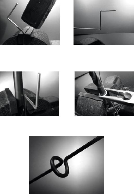
3.
Draw another line at a
distance of 3.6 cm from the
bend. Using the
vice
and
the hammer, bend once
again the wire over
this second line at
90
degrees,
in the opposite direction to
the first
bend but in the same
plane.
The
wire should look like a
Z
.
120
Chapter
4: Antennas & Transmission
Lines
Figure
4.16: Bend the wire
into a "Z" shape.
4.
We will now twist the
Z portion of
the wire to make a coil
with a diameter
of
1 cm. To do this, we will
use the pipe or the
drill bit and curve
the wire
around
it, with the help of
the vice and of the
pliers.
Figure
4.17: Bend the wire
around the drill bit to make
a coil.
The
coil will look like
this:
Figure
4.18: The completed
coil.
5.
You should make a second
coil at a distance of 7.8 cm
from the first
one.
Both
coils should have the
same turning direction and
should be placed
on
the same side of the
wire. Make a third and a
fourth coil following
the
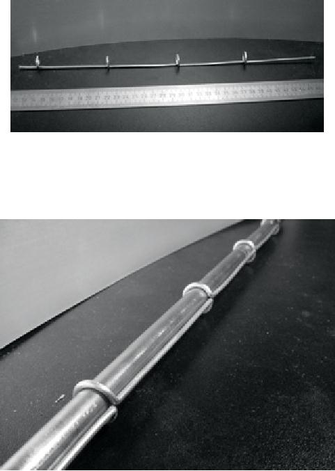
Chapter
4: Antennas & Transmission
Lines
121
same
procedure, at the same
distance of 7.8 cm one from
each other.
Trim
the last phased element at a
distance of 8.0 cm from the
fourth coil.
Figure
4.19: Try to keep it as
straight possible.
If
the coils have been
made correctly, it should
now be possible to insert
a
pipe
through all the coils as
shown.
Figure
4.20: Inserting a pipe can
help to straighten the
wire.
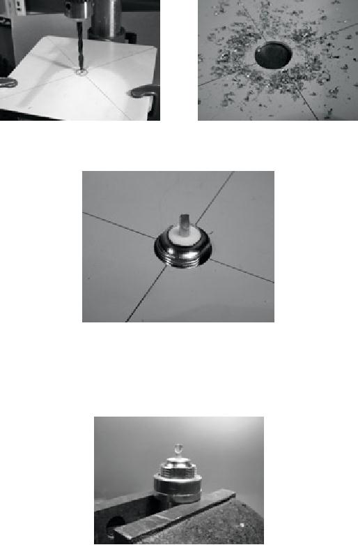
6.
With a marker and a ruler,
draw the diagonals on the
metallic plate, find-
ing
its center. With a small
diameter drill bit, make a
pilot hole at the
cen-
ter
of the plate. Increase the
diameter of the hole using
bits with an in-
creasing
diameter.
122
Chapter
4: Antennas & Transmission
Lines
Figure
4.21: Drilling the hole in
the metal plate.
The
hole should fit the N
connector exactly. Use a file
if needed.
Figure
4.22: The N connector should
fit
snugly in the
hole.
7.
To have an antenna impedance of 50
Ohms, it is important that
the visi-
ble
surface of the internal
insulator of the connector
(the white area
around
the central pin) is at the
same level as the surface of
the plate.
For
this reason, cut 0.5 cm of
copper pipe with an external
diameter of 2
cm,
and place it between the
connector and the
plate.
Figure
4.23: Adding a copper pipe
spacer helps to match the
impedance of the
an-
tenna
to 50 Ohms.
Chapter
4: Antennas & Transmission
Lines
123
8.
Screw the nut to the
connector to fix it firmly on the plate
using the spanner.
Figure
4.24: Secure the N connector
tightly to the
plate.
9.
Smooth with the file the
side of the wire which is
2.5 cm long, from
the
first
coil. Tin the wire
for around 0.5 cm at the
smoothed end helping
yourself
with the vice.
Figure
4.25: Add a little solder to
the end of the wire to
"tin" it prior to
soldering.
10.
With the soldering iron,
tin the central pin of
the connector. Keeping
the
wire
vertical with the pliers,
solder its tinned side in
the hole of the
central
pin.
The first
coil should be at 3.0 cm
from the plate.
124
Chapter
4: Antennas & Transmission
Lines
Figure
4.26: The first
coil should start 3.0 cm
from the surface of the
plate.
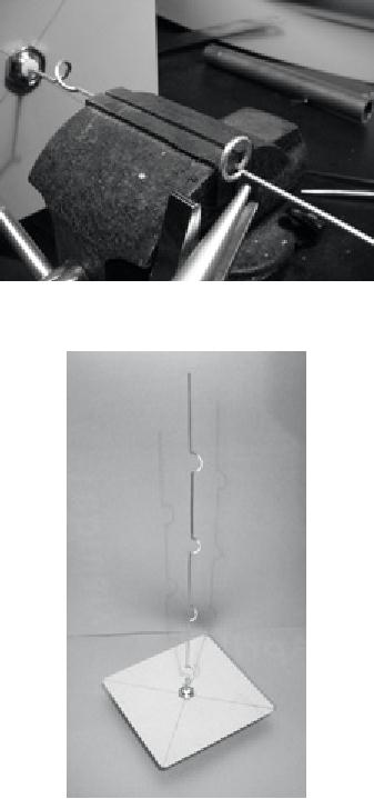
11.
We are now going to stretch
the coils extending the
total vertical length
of
the
wire. Using the use
the vice and the
pliers, you should pull
the cable
so
that the final
length of the coil is of 2.0
cm.
Figure
4.27: Stretching the coils.
Be very gentle and try
not to scrape the surface
of
the
wire with the
pliers.
12.
Repeat the same procedure
for the other three
coils, stretching
their
length
to 2.0 cm.
Chapter
4: Antennas & Transmission
Lines
125
Figure
4.28: Repeat the stretching
procedure for all of the
remaining coils.
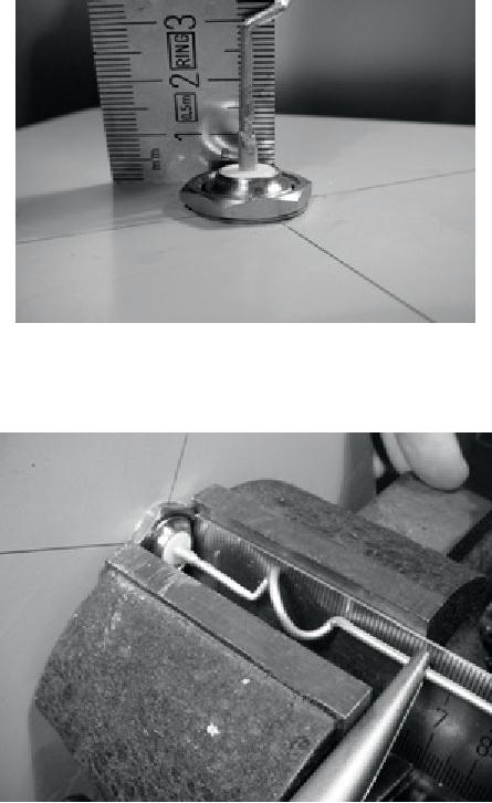
13.
At the end the antenna
should measure 42.5 cm from
the plate to the
top.
Figure
4.29: The finished
antenna should be 42.5 cm
from the plate to the
end of the
wire.
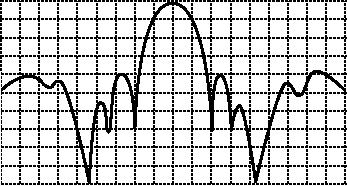
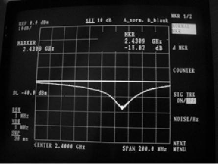
14.
If you have a spectrum
analyzer with a tracking
generator and a
direc-
tional
coupler, you can check
the curve of the reflected
power of the an-
tenna.
The picture below shows
the display of the spectrum
analyzer.
126
Chapter
4: Antennas & Transmission
Lines
Figure
4.30: A spectrum plot of the
reflected
power of the collinear
omni.
If
you intend to use this
antenna outside, you will
need to weatherproof
it.
The
simplest method is to enclose
the whole thing in a large
piece of PVC
pipe
closed with caps. Cut a
hole at the bottom for
the transmission line,
and
seal
the antenna shut with
silicone or PVC glue.
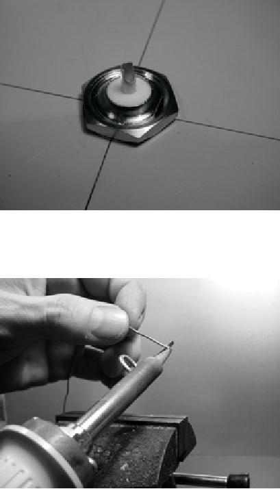
Cantenna
The
waveguide antenna, sometimes
called a Cantenna, uses a
tin can as a
waveguide
and a short wire soldered on
an N connector as a probe
for
coaxial-cable-to-waveguide
transition. It can be easily
built at just the price
of
the
connector, recycling a food,
juice, or other tin can. It
is a directional an-
tenna,
useful for short to medium
distance point-to-point links. It
may be also
used
as a feeder for a parabolic
dish or grid.
Not
all cans are good
for building an antenna
because there are
dimensional
constraints.
1.
The acceptable values for
the diameter D of the feed
are between 0.60
and
0.75 wavelength in air at
the design frequency. At
2.44 GHz the
wavelength
is 12.2 cm, so the can
diameter should be in the
range of
7.3
- 9.2 cm.
2.
The length L of the can
preferably should be at least
0.75 G
,
where G
is
the guide wavelength and is
given by:
Chapter
4: Antennas & Transmission
Lines
127
G
=
/
1.706D)2)
sqrt(1
- (
For
D = 7.3 cm, we need a can of
at least 56.4 cm, while
for D = 9.2 cm we
need
a can of at least 14.8 cm.
Generally the smaller the
diameter, the longer
the
can should be. For
our example, we will use
oil cans that have a
diameter
of
8.3 cm and a height of about
21 cm.
3.
The probe for coaxial
cable to waveguide transition
should be positioned
at
a distance S from the bottom
of the can, given
by:
S
= 0.25
G
Its
length should be 0.25 ,
which at
2.44 GHz corresponds to 3.05
cm.
L
S
D
Figure
4.31: Dimensional constraints on
the cantenna
The
gain for this antenna
will be in the order of 10 to 14
dBi, with a beam-
width
of around 60 degrees.

128
Chapter
4: Antennas & Transmission
Lines
Figure
4.32: The finished
cantenna.
Parts
list
·
one screw-on N-type female
connector
·
4 cm of copper or brass wire of 2 mm of
diameter
·
an oil can of 8.3 cm of
diameter and 21 cm of
height
Figure
4.33: Parts needed for
the can antenna.

Chapter
4: Antennas & Transmission
Lines
129
Tools
required
·
Can opener
·
Ruler
·
Pliers
·
File
·
Soldering iron
·
Solder
·
Drill with a set of bits
for metal (with a 1.5 cm
diameter bit)
·
Vice or clamp
·
Spanner or monkey
wrench
·
Hammer
·
Punch
Construction
1.
With the can opener,
carefully remove the upper
part of the can.
Figure
4.34: Be careful of sharp
edges when opening the
can.
The
circular disk has a very
sharp edge. Be careful when
handling it! Empty
the
can and wash it with
soap. If the can contained
pineapple, cookies, or
some
other tasty treat, have a
friend serve the
food.
2.
With the ruler, measure
6.2 cm from the bottom of
the can and draw
a
point.
Be careful to measure from
the inner side of the
bottom. Use a
punch
(or a small drill bit or a
Phillips screwdriver) and a
hammer to mark
the
point. This makes it easier
to precisely drill the hole.
Be careful not to
130
Chapter
4: Antennas & Transmission
Lines
change
the shape of the can
doing this by inserting a
small block of
wood
or other object in the can
before tapping it.
Figure
4.35: Mark the hole
before drilling.
3.
With a small diameter drill
bit, make a hole at the
center of the plate.
In-
crease
the diameter of the hole
using bits with an
increasing diameter.
The
hole should fit exactly
the N connector. Use the
file to smooth
the
border
of the hole and to remove
the painting around it in
order to ensure
a
better electrical contact
with the connector.
Figure
4.36: Carefully drill a
pilot hole, then use a
larger bit to finish
the job.
4.
Smooth with the file one
end of the wire. Tin
the wire for around
0.5 cm
at
the same end helping
yourself with the
vice.
Chapter
4: Antennas & Transmission
Lines
131
Figure
4.37: Tin the end of
the wire before
soldering.
5.
With the soldering iron,
tin the central pin of
the connector. Keeping
the
wire
vertical with the pliers,
solder its tinned side in
the hole of the
cen-
tral
pin.
Figure
4.38: Solder the wire to
the gold cup on the N
connector.
6.
Insert a washer and gently
screw the nut onto
the connector. Trim
the
wire
at 3.05 cm measured from the
bottom part of the
nut.
132
Chapter
4: Antennas & Transmission
Lines
Figure
4.39: The length of the
wire is critical.
7.
Unscrew the nut from
the connector, leaving the
washer in place.
Insert
the
connector into the hole of
the can. Screw the
nut on the connector
from
inside the can.
Figure
4.40: Assemble the
antenna.
8.
Use the pliers or the
monkey wrench to screw firmly
the nut on the
con-
nector.
You are done!
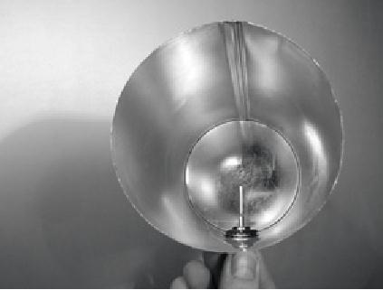
Chapter
4: Antennas & Transmission
Lines
133
Figure
4.41: Your finished
cantenna.
As
with the other antenna
designs, you should make a
weatherproof enclo-
sure
for the antenna if you
wish to use it outdoors. PVC
works well for
the
can
antenna. Insert the entire
can in a large PVC tube,
and seal the
ends
with
caps and glue. You
will need to drill a hole in
the side of the tube to
ac-
commodate
the N connector on the side
of the can.
Cantenna
as dish feed
As
with the USB dongle
parabolic, you can use
the cantenna design as
a
feeder
for significantly
higher gain. Mount the
can on the parabolic with
the
opening
of the can pointed at the
center of the dish. Use
the technique de-
scribed
in the USB dongle antenna
example (watching signal
strength
changes
over time) to find the
optimum location of the can
for the dish
you
are
using.
By
using a well-built cantenna
with a properly tuned
parabolic, you can
achieve
an overall antenna gain of
30dBi or more. As the size
of the para-
bolic
increases, so does the
potential gain and
directivity of the
antenna.
With
very large parabolas, you
can achieve significantly
higher gain.
For
example, in 2005, a team of
college students successfully
established a
link
from Nevada to Utah in the
USA. The link crossed a
distance of over
200
kilometers! The wireless
enthusiasts used a 3.5 meter
satellite dish to
establish
an 802.11b link that ran at
11 Mbps,
without using an amplifier.
De-
tails
about this achievement can
be found at http://www.wifi-shootout.com/
134
Chapter
4: Antennas & Transmission
Lines
NEC2
NEC2
stands
for Numerical
Electromagnetics Code (version 2)
and is a
free
antenna modeling package.
NEC2 lets you build an
antenna model in
3D,
and then analyzes the
antenna s
electromagnetic
response. It was de-
veloped
more than ten years
ago and has been
compiled to run on
many
different
computer systems. NEC2 is
particularly effective for
analyzing wire-
grid
models, but also has
some surface patch modeling
capability.
The
antenna design is described in a
text file,
and then the model is
built us-
ing
this text description. An
antenna described in NEC2 is
given in two parts:
its
structure
and a
sequence of controls. The
structure is simply a
numeri-
cal
description of where the
different parts of the
antenna are located,
and
how
the wires are connected
up. The controls tell
NEC where the RF
source
is
connected. Once these are
defined,
the transmitting antenna is
then mod-
eled.
Because of the reciprocity
theorem the transmitting
gain pattern is the
same
as the receiving one, so
modeling the transmission
characteristics is
sufficient
to understand the antenna's
behavior completely.
A
frequency or range of frequencies of
the RF signal must be
specified.
The
next
important element is the
character of the ground. The
conductivity of the
earth
varies from place to place,
but in many cases it plays a
vital role in de-
termining
the antenna gain
pattern.
To
run NEC2 on Linux, install
the NEC2 package from
the URL below. To
launch
it, type nec2
and
enter the input and
output filenames. It is
also worth
installing
the xnecview
package
for structure verification
and radiation pat-
tern
plotting. If all went well
you should have a file containing
the output. This
can
be broken up into various
sections, but for a quick
idea of what it
repre-
sents
a gain pattern can be
plotted using xnecview. You
should see the
ex-
pected
pattern, horizontally omnidirectional,
with a peak at the optimum
an-
gle
of takeoff. Windows and Mac
versions are also
available.
The
advantage of NEC2 is that we
can get an idea of how
the antenna works
before
building it, and how we
can modify the design in
order to get the
maximum
gain. It is a complex tool
and requires some research
to learn how
to
use it effectively, but it is an
invaluable tool for antenna
designers.
NEC2
is available from http://www.nec2.org/
Online
documentation can be obtained
from the "Unofficial
NEC Home Page"
at
http://www.nittany-scientific.com/nec/
.
Table of Contents:
- Where to Begin:Purpose of this book, Fitting wireless into your existing network, Wireless networking protocols
- A Practical Introduction to Radio Physics:What is a wave?, Polarization
- Network Design:Designing the physical network, Mesh networking with OLSR, Estimating capacity
- Antennas & Transmission Lines:Cables, Waveguides, Connectors and adapters, Amplifiers
- Networking Hardware:Wired wireless, Choosing wireless components, Building an access point from a PC
- Security & Monitoring:Physical security, Threats to the network, Authentication
- Solar Power:Solar energy, Photovoltaic system components, The battery
- Building an Outdoor Node:Waterproof enclosures, Providing power, Mounting considerations
- Troubleshooting:Building your team, Proper troubleshooting technique, Common network problems
- Economic Sustainability:Create a Mission Statement, Evaluate the Demand for Potential Offerings
- Case Studies:General advice, Crossing the divide with a simple bridge in Timbuktu, Networking Mérida State
- Appendix A: Resources:Antennas and antenna design, Security
- Appendix B: Channel Allocations
- Appendix C: Path Loss
- Appendix D: Cable Sizes
- Appendix E: Solar Dimensioning:General Data, Component Characteristics
- Glossary