Security Market Line, Capital Asset Pricing Model – CAPM Calculating Over, Under valued stocks

<< Portfolio and Diversification, Portfolio and Variance, Risk–Systematic & Unsystematic, Beta – Measure of systematic risk, Aggressive & defensive stocks

Cost of Capital & Capital Structure, Components of Capital, Cost of Equity, Estimating g or growth rate, Dividend growth model, Cost of Debt, Bonds, Cost of Preferred Stocks >>

Corporate Finance FIN 622

Lesson 17

SECURITIES MARKET LINE & CAPITAL ASSET PRICING MODEL CAPM

The following topics will be discussed in this lecture.

Security Market Line

Capital Asset Pricing Model CAPM

Calculating Over/Under valued stocks

SECURITIES MARKET LINE:

The security market line tells us how risk is rewarded in the market. Let's assume that expected return (Er)

on any asset is Erm is 18% and beta of 1.5 and risk free rate (Rf) is 8%. Please note a risk free asset has a

beta of zero because it has no systematic risk.

Going forward, we create a portfolio comprising of an Asset A and risk free asset. We calculate expected

return on portfolio by changing the investment level in both assets. For example, if 30% of the investment

is made in asset A, the expected return will be

E(r) = %a x E(r) A + %b x Rf

E(r) = 30% x 18% + (1 - 0.30) x 8%

= 5.40 + 6 = 11.40%

And the beta of this portfolio can be computed as:

Bp = 30% x Ba + 70% x Bb

Bp = 0.30 x 1.50 + 70% x 0 (since risk-free asset has zero beta)

Bp = 0.45 + 0 = 0.45

Now you can think that can we increase our investment in stock A beyond 100% level. This can be done by

if the investor borrows at risk free rate. Assuming that investment in stock A is increased to 150% and this

would imply that investment in risk free asset has been reduced by 50% in order to keep investment at

100% level.

The expected return on this portfolio will be:

Er (p) = 1.50 x 18% + -0.50 x 8%

= 27 % - 4% = 23%

The portfolio beta will be:

B (p) = 1.5 x 150% + (100 -150) x 0

= 2.25 + 0 = 2.25

Now we can work out different investment possibilities by changing the portion of amount invested in asset

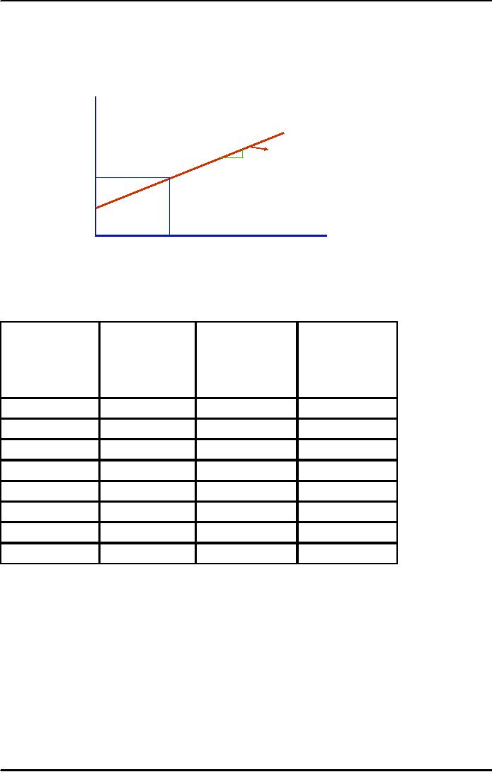
A. Also, we plot these values to draw a graph.

Corporate Finance FIN 622

Portfolio Expected Return

Investment in A

ERa Rf/ Beta

ERa

18%

Slope = 6.67

Rf=8%

1.50

Portfolio Beta

% OF

PORTFOLIO

INVESTMENT

PORTFOLIO

IN STOCK A

BETA

CURVE SLOPE

8.00

10.50

0.3750

6.67

13.00

0.7500

6.67

15.50

1.1250

6.67

100

18.00

1.5000

6.67

125

20.50

1.8750

6.67

150

23.00

2.2500

6.67

Reward to Risk = (ER a - ER rf) / BETA a

= 0.0666667 or 6.67

The graph and table tell us something clearly that slop of the curve returns a constant value at all investment

levels. The slop of curve is just the risk premium on assets A divided by Asset A's beta Ba.

Slope of curve = Era Rf / Ba (18 8)/1.5 = 6.667

The fourth column in the table uses this formula to calculate the slop.

Now we advance our example and consider another asset B, offering expected return of 14% and a beta of

1.10. The Rf is the same i.e., 8%.

Assuming that we invest 30% in asset B and rest in risk free asset. Then portfolio return can be calculated

the way we did above.

That is

Erp = .30 x 14% + (1 - .30) x 8%

= 4.2 + 5.6 = 9.80%

Portfolio beta is

Corporate Finance FIN 622

Bp = .30 x 1.10 + .70 x 0

= 0.33

Like asset A, we can work out different investment combination and a graph as under:

Portfolio Expected Return

Investment in B

ERa Rf/ Beta

ERa

14%

Slope= 5.45

Rf=8%

1.10

Portfolio Beta

% OF

PORTFOLIO

CURVE SLOPE

INVESTMENT

BETA

IN STOCK A

8.00

9.50

0.28

5.45

11.00

0.55

5.45

12.50

0.83

5.45

100

14.00

1.10

5.45

125

15.50

1.38

5.45

150

17.00

1.65

5.45

Reward to Risk = (ER a - ER rf) / BETA a

= 5.45

The risk to reward ratio of 5.45% is returned by the stock B and is less than the return offered by stock A.

It is clear from the example that stock A is offering more returns than stock B. In a well organized market

this situation will not persist for a long period of time. This is because more investors will invest in stock A

and at the same time investment in stock B will reduce. This situation will push up the price of stock A

resulting in reduction in returns of this stock. The prices of stock B will reduce thereby increase the returns.

This situation will continue till the point when the prices of both assets are same. Thus in an efficient

market the slope of both assets will be the same.

Era Rf/Ba = Erb Rf/Bb

Moving towards the conclusions that regardless of number of assets available in the market, the reward to

risk ratio must the same for all the stocks available in the market.

Corporate Finance FIN 622

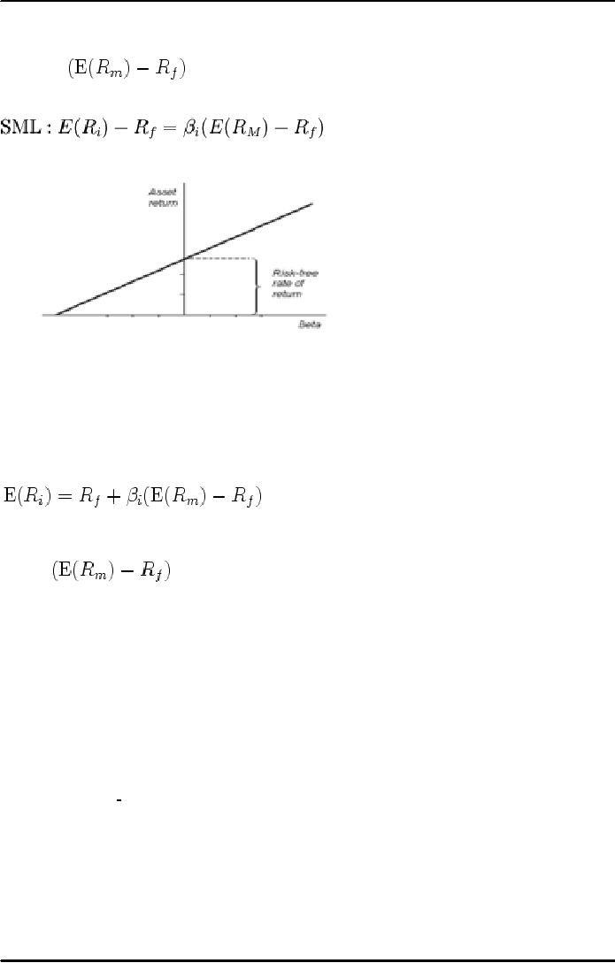
The relationship between Beta & required return is plotted on the securities market line (SML) which

shows expected return as a function of β. The intercept is the risk-free rate available for the market, while

. The Securities market line can be regarded as representing a single-factor

the slope is

model of the asset price, where Beta is exposure to changes in value of the Market. The equation of the

SML is thus:

The Security Market Line

CAPITAL ASSET PRICING MODEL:

The asset return depends on the amount paid for the asset today. The price paid must ensure that the

market portfolio's risk / return characteristics improve when the asset is added to it. The CAPM is a model

which derives the theoretical required return (i.e. discount rate) for an asset in a market, given the risk-free

rate available to investors and the risk of the market as a whole.

The CAPM is usually expressed:

β, Beta, is the measure of asset sensitivity to a movement in the overall market; Beta is usually

found via regression on historical data. Betas exceeding one signify more than average "riskiness"; betas

below one indicate lower than average.

is the market premium, the historically observed excess return of the market

over the risk-free rate.

Once the expected return, E(ri), is calculated using CAPM, the future cash flows of the asset can be

discounted to their present value using this rate to establish the correct price for the asset. (Here again, the

theory accepts in its assumptions that a parameter based on past data can be combined with a future expectation.)

A more risky stock will have a higher beta and will be discounted at a higher rate; less sensitive stocks will

have lower betas and be discounted at a lower rate. In theory, an asset is correctly priced when its observed

price is the same as its value calculated using the CAPM derived discount rate. If the observed price is

higher than the valuation, then the asset is overvalued; it is undervalued for a too low price. Summarizing

this discussion we can say that CAPM tell us:

Time value of money: risk free rate "Rf" is a rate when you don't take risk. it is just waiting

for money.

Reward for risk: the equation "Erm Rf" represents reward for taking average systematic

risk in addition to waiting.

Systematic risk: is measured by beta. This measure the systematic risk present in an assets

or portfolio, relative to average asset.

Calculating Over/Under Valued Stocks

An asset is said to be overvalued if its price is much higher given its expected return and risk. On the other

hand, an asset is said to be undervalued if its price is much lower given its Er and risk.

Corporate Finance FIN 622

Risk to

Reward

STOCK

BETA

Ratio

ABC

1.5

5.33

XYZ

0.9

4.44

Risk Free Rate

SLOPE OF SML:

ERa Rf/ Beta

ABC

5.33

XYZ

4.44

Consider the above example where we have two assets and their expected return and beta is given. We also

calculate the risk-to-reward ratio assuming the risk free rate of 7%.

We can conclude that XYZ offers an insufficient expected return given its level of risk relative to ABC. This

is because former's expected returns are very low and its price is high. Therefore, XYZ is overvalued

relative to ABC. In efficient market the price of this stock will fall. On the same we can say that ABC is

undervalued stock and its price will rise.

Table of Contents: