 |

Database
Management System
(CS403)
VU
Lecture No.
17
Reading
Material
"Database
Systems Principles, Design
and Implementation"
Chapter
6
written
by Catherine Ricardo, Maxwell
Macmillan.
Overview of Lecture:
o Five
Basic Operators of Relational
Algebra
o Join
Operation
In the
previous lecture we discussed
about the transformation of
conceptual database
design
into relational database. In
E-R data model we had number
of constructs but in
relational
data model it was only a
relation or a table. We started discussion on
data
manipulation
languages (DML) of relational data model
(SDM). We will now
study
in detail
the different operators
being used in relational
algebra.
The
relational algebra is a procedural
query language. It consists of a
set of operations
that
take one or two relations as
input and produce a new
relation as their result.
There
are
five basic operations of relational
algebra. They are broadly
divided into two
categories:
Unary
Operations:
These
are those operations, which
involve only one relation or
table. These are Select
and
Project
Binary
Operations:
These
are those operations, which
involve pairs of relations
and are, therefore
called
as binary
operations. The input for
these operations is two
relations and they
produce
a new
relation without changing
the original relations.
These operations are:
o Union
148

Database
Management System
(CS403)
VU
o Set
Difference
o Cartesian
Product
The
Select Operation:
The
select operation is performed to select
certain rows or tuples of a
table, so it
performs
its action on the table
horizontally. The tuples are
selected through this
operation
using a predicate or condition.
This command works on a
single table and
takes
rows that meet a specified
condition, copying them into
a new table. Lower
Greek
letter sigma (σ) is used
to denote the selection. The
predicate appears as
subscript
to σ. The
argument relation is given in parenthesis
following theσ. As
a
result of
this operation a new table
is formed, without changing
the original table.
As
a result
of this operation all the
attributes of the resulting
table are same, which
means
that
degree of the new and old
tables are same. Only
selected rows / tuples are
picked
up by the
given condition. While processing a
selection all the tuples of
a table are
looked up
and those tuples, which
match a particular condition,
are picked up for
the
new
table. The degree of the
resulting relation will be
the same as of the relation
itself.
| σ | = |
r(R) |
The
select operation is commutative,
which is as under: -
σc1
(σc2(R)) = σc2
(σc1(R))
If a
condition 2 (c2) is applied on a
relation R and then c1 is
applied, the
resulting
table
would be equivalent even if
this condition is reversed that is
first c1 is applied
and
then c2 is applied.
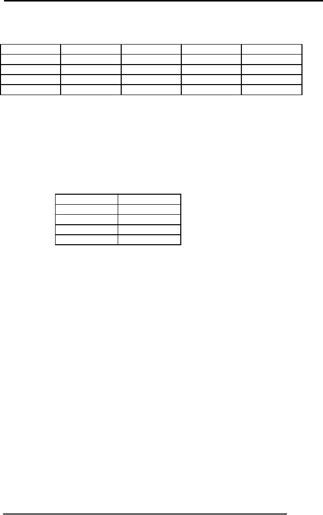
For
example there is a table
STUDENT with five
attributes.
STUDENT
stId
stName
stAdr
prName
curSem
S1020
Sohail
Dar
H#14,
F/8-4,Islamabad.
MCS
4
S1038
Shoaib
Ali
H#23,
G/9-1,Islamabad
BCS
3
S1015
Tahira
Ejaz
H#99,
Lala Rukh Wah.
MCS
5
S1018
Arif
Zia
H#10,
E-8, Islamabad.
BIT
5
149

Database
Management System
(CS403)
VU
Fig. 1:
An example STDUDENT
table
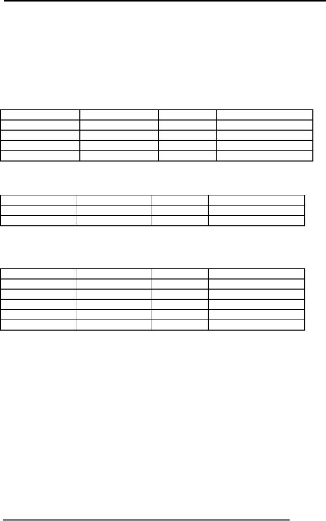
The
following is an example of select
operation on the table
STUDENT:
σ Curr_Sem > 3
(STUDENT)
σ
is
the
The
components of the select operations are
clear from the above
example;
symbol
being used (operato),
"curr_sem > 3" written in the
subscript is the
predicate
and
STUDENT given in parentheses is
the table name. The
resulting relation of
this
command
would contain record of those students
whose semester is greater than
three
as
under:
σ Curr_Sem > 3
(STUDENT)
stId
stName
stAdr
prName
curSem
S1020
Sohail
Dar
H#14,
F/8-4,Islamabad.
MCS
4
S1015
Tahira
Ejaz H#99, Lala Rukh
Wah.
MCS
5
S1018
Arif
Zia
H#10,
E-8, Islamabad.
BIT
5
Fig. 2:
Output relation of a select
operation
In
selection operation the
comparison operators like <, >, =,
<=, >=, <> can be
used in
the
predicate. Similarly, we can also
combine several simple predicates
into a larger
predicate
using the connectives and
(∧) and
or
(∨). Some
other examples of
select
operation
on the STUDENT table are
given below:
σ stId = `S1015'
(STUDENT)
σ prName <> `MCS'
(STUDENT)
The
Project Operator
The
Select operation works horizontally on
the table on the other
hand the Project
operator
operates on a single table vertically,
that is, it produces a vertical
subset of
the
table, extracting the values
of specified columns, eliminating
duplicates, and
placing
the values in a new table.
It is unary operation that
returns its argument
relation,
with certain attributes left
out. Since relation is a set
any duplicate rows
are
eliminated.
Projection is denoted by a Greek
letter (∏). While
using this operator
all
the
rows of selected attributes of a relation
are part of new relation.
For example
consider
a relation FACULTY with five
attributes and certain
number of rows.
150
Database
Management System
(CS403)
VU
FACULTY
FacId
facName
Dept
Salary
Rank
F2345
Usman
CSE
21000
lecturer
F3456
Tahir
CSE
23000
Asst
Prof
F4567
Ayesha
ENG
27000
Asst
Prof
F5678
Samad
MATH
32000
Professor
Fig. 3:
An example FACULY table
If we
apply the projection
operator on the table for
the following commands all
the
rows of
selected attributes will be shown, for
example:
∏
(FACULTY)
FacId,
Salary
FacId
Salary
F2345
21000
F3456
23000
F4567
27000
F5678
32000
Fig. 4:
Output relation of a project
operation on table of figure
3
Some
other examples of project
operation on the same table
can be:
∏ Fname,
Rank (Faculty)
∏ Facid,
Salary,Rank (Faculty)
151

Database
Management System
(CS403)
VU
Composition
of Relational Operators:
The
relational operators like
select and project can also
be used in nested
forms
iteratively.
As the result of an operation is a
relation so this result can
be used as an
input
for other operation. For
Example if we want the names
of faculty members
along
with departments, who are
assistant professors then we have to
perform both the
select
and project operations on
the FACULTY table of figure 3.
First selection
operator
is applied for selecting the
associate professors, the operation
outputs a
relation
that is given as input to
the projection operation for
the required
attributes.
∏ facName,
dept (σ rank='Asst Prof'
(FACULTY))
The
output of this command will
be
facName
Dept
Tahir
CSE
Ayesha
ENG
Fig. 5:
Output relation of nested
operations' command
We have
to be careful about the
nested command sequence. For
example in the above
nested
operations example, if we change the
sequence of operations and
bring the
projection
first then the relation
provided to select operation as
input will not have
the
attribute
of rank and so then
selection operator can't be
applied, so there would be
an
error. So
although the sequence can be
changed, but the required
attributes should be
there
either for selection or
projection.
The
Union Operation:
We will
now study the binary
operations, which are also
called as set operations.
The
first
requirement for union
operator is that the both
the relations should be
union
compatible.
It means that relations must meet
the following two
conditions:
·
Both
the relations should be of
same degree, which means
that the number of
attributes
in both relations should be
exactly same
·
The
domains of corresponding attributes in
both the relations should be
same.
Corresponding
attributes means first
attributes of both relations,
then second and so
on.
It is
denoted by U. If R and S are
two relations, which are
union compatible, if we
take
union of these two relations
then the resulting relation
would be the set of
tuples
either in
R or S or both. Since it is set so
there are no duplicate
tuples. The union
operator
is commutative which means:
-
152
Database
Management System
(CS403)
VU
RUS=SUR
For
Example there are two
relations COURSE1 and
COURSE2 denoting the
two
tables
storing the courses being
offered at different campuses of an
institute? Now if
we want
to know exactly what courses
are being offered at both
the campuses then we
will take
the union of two
tables:
COURSE1
crId
progId
credHrs
courseTitle
C2345
P1245
3
Operating
Sytems
C3456
P1245
4
Database
Systems
C4567
P9873
4
Financial
Management
C5678
P9873
3
Money
& Capital Market
COURSE2
crId
progId
credHrs
courseTitle
C4567
P9873
4
Financial
Management
C8944
P4567
4
Electronics
COURSE1 U
COURSE2
crId
progId
credHrs
courseTitle
C2345
P1245
3
Operating
Sytems
C3456
P1245
4
Database
Systems
C4567
P9873
4
Financial
Management
C5678
P9873
3
Money
& Capital Market
C8944
P4567
4
Electronics
Fig. 5:
Two tables and output of
union operation on those tables
So in the
union of above two courses
there are no repeated tuples and
they are union
compatible
as well
153
Database
Management System
(CS403)
VU
The
Intersection Operation:
The
intersection operation also
has the requirement that
both the relations should
be
union
compatible, which means they
are of same degree and same
domains. It is
represented
by∩. If R
and S are two relations
and we take intersection of
these two
relations
then the resulting relation
would be the set of tuples,
which are in both R
and
S. Just
like union intersection is also
commutative.
R∩S=S∩R
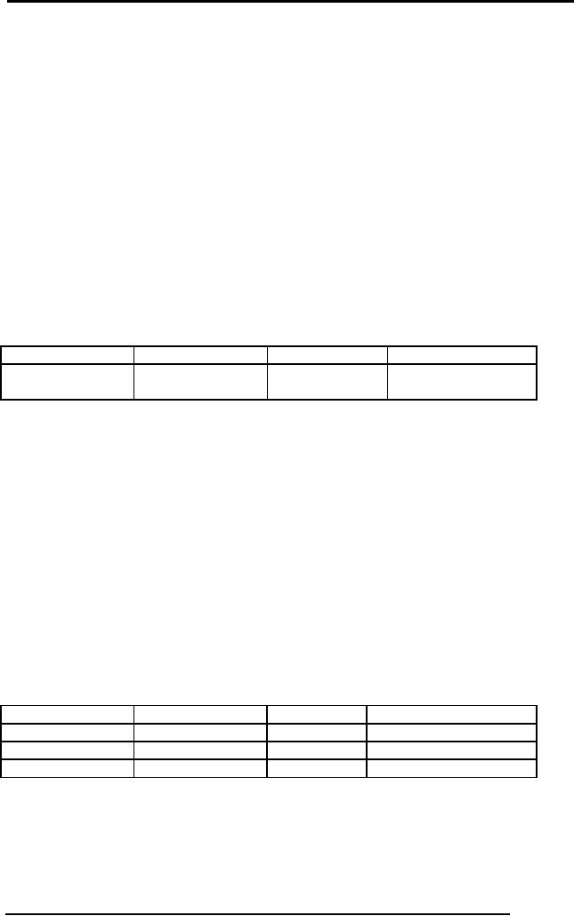
For
Example, if we take intersection of
COURSE1 and COURSE2 of
figure 5 then
the
resulting relation would be
set of tuples, which are
common in both.
COURSE1
∩
COURSE2
crId
progId
credHrs
courseTitle
C4567
P9873
4
Financial
Management
Fig. 6:
Output of intersection operation on
COURSE1 and COURSE 2 tables of
figure
5
The
union and intersection operators are
used less as compared to selection
and
projection
operators.
The
Set Difference
Operator:
If R and
S are two relations which
are union compatible then
difference of these
two
relations
will be set of tuples that appear in R
but do not appear in S. It is denoted
by
(-)
for example if we apply
difference operator on Course1 and
Course2 then the
resulting
relation would be as
under:
COURSE1
COURSE2
CID
ProgID
Cred_Hrs
CourseTitle
C2345
P1245
3
Operating
Sytems
C3456
P1245
4
Database
Systems
C5678
P9873
3
Money
& Capital Market
Fig. 7:
Output of difference operation on
COURSE1 and COURSE 2 tables
of figure
5
Cartesian
product:
154

Database
Management System
(CS403)
VU
The
Cartesian product needs not
to be union compatible. It means
they can be of
different
degree. It is denoted by X. suppose there
is a relation R with attributes
(A1,
A2,...An)
and S with attributes (B1,
B2......Bn). The Cartesian
product will be:
RX
S
The
resulting relation will be containing
all the attributes of R and
all of S. Moreover,
all
the rows of R will be merged
with all the rows of S. So
if there are m attributes
and
C rows in
R and n attributes and D
rows in S then the relations
R x S will contain m +
n columns
and C * D rows. It is also called as
cross product. The Cartesian
product is
also
commutative and associative.
For Example there are
two relations COURSE
and
STUEDNT
COURSE
STUDENT
crId
courseTitle
stId
stName
C3456
Database
Systems
S101
Ali
Tahir
C4567
Financial
Management
S103
Farah
Hasan
C5678
Money
& Capital Market
COURSE X
STUDENT
crId
courseTitle
stId
stName
C3456
Database
Systems
S101
Ali
Tahir
C4567
Financial
Management
S101
AliTahr
C5678
Money
& Capital Market
S101
Ali
Tahir
C3456
Database
Systems
S103
Farah
Hasan
C4567
Financial
Management
S103
Farah
Hasan
C5678
Money
& Capital Market
S103
Farah
Hasan
Fig. 7:
Input tables and output of
Cartesian product
Join
Operation:
Join is a
special form of cross
product of two tables. In
Cartesian product we join
a
tuple of
one table with the
tuples of the second table.
But in join there is a
special
requirement
of relationship between tuples.
For example if there is a
relation
STUDENT
and a relation BOOK then it
may be required to know that
how many
books
have been issued to any
particular student. Now in
this case the primary
key of
STUDENT
that is stId is a foreign
key in BOOK table through
which the join can
be
made. We will
discuss in detail the
different types of joins in
our next lecture.
155

Database
Management System
(CS403)
VU
In this
lecture we discussed different
types of relational algebra
operations. We will
continue
our discussion in the next
lecture.
156
Table of Contents:
- Introduction to Databases and Traditional File Processing Systems
- Advantages, Cost, Importance, Levels, Users of Database Systems
- Database Architecture: Level, Schema, Model, Conceptual or Logical View:
- Internal or Physical View of Schema, Data Independence, Funct ions of DBMS
- Database Development Process, Tools, Data Flow Diagrams, Types of DFD
- Data Flow Diagram, Data Dictionary, Database Design, Data Model
- Entity-Relationship Data Model, Classification of entity types, Attributes
- Attributes, The Keys
- Relationships:Types of Relationships in databases
- Dependencies, Enhancements in E-R Data Model. Super-type and Subtypes
- Inheritance Is, Super types and Subtypes, Constraints, Completeness Constraint, Disjointness Constraint, Subtype Discriminator
- Steps in the Study of system
- Conceptual, Logical Database Design, Relationships and Cardinalities in between Entities
- Relational Data Model, Mathematical Relations, Database Relations
- Database and Math Relations, Degree of a Relation
- Mapping Relationships, Binary, Unary Relationship, Data Manipulation Languages, Relational Algebra
- The Project Operator
- Types of Joins: Theta Join, EquiJoin, Natural Join, Outer Join, Semi Join
- Functional Dependency, Inference Rules, Normal Forms
- Second, Third Normal Form, Boyce - Codd Normal Form, Higher Normal Forms
- Normalization Summary, Example, Physical Database Design
- Physical Database Design: DESIGNING FIELDS, CODING AND COMPRESSION TECHNIQUES
- Physical Record and De-normalization, Partitioning
- Vertical Partitioning, Replication, MS SQL Server
- Rules of SQL Format, Data Types in SQL Server
- Categories of SQL Commands,
- Alter Table Statement
- Select Statement, Attribute Allias
- Data Manipulation Language
- ORDER BY Clause, Functions in SQL, GROUP BY Clause, HAVING Clause, Cartesian Product
- Inner Join, Outer Join, Semi Join, Self Join, Subquery,
- Application Programs, User Interface, Forms, Tips for User Friendly Interface
- Designing Input Form, Arranging Form, Adding Command Buttons
- Data Storage Concepts, Physical Storage Media, Memory Hierarchy
- File Organizations: Hashing Algorithm, Collision Handling
- Hashing, Hash Functions, Hashed Access Characteristics, Mapping functions, Open addressing
- Index Classification
- Ordered, Dense, Sparse, Multi-Level Indices, Clustered, Non-clustered Indexes
- Views, Data Independence, Security, Vertical and Horizontal Subset of a Table
- Materialized View, Simple Views, Complex View, Dynamic Views
- Updating Multiple Tables, Transaction Management
- Transactions and Schedules, Concurrent Execution, Serializability, Lock-Based Concurrency Control, Deadlocks
- Incremental Log with Deferred, Immediate Updates, Concurrency Control
- Serial Execution, Serializability, Locking, Inconsistent Analysis
- Locking Idea, DeadLock Handling, Deadlock Resolution, Timestamping rules