 |
Online Analytical Processing OLAP: DWH and OLAP, OLTP |
| << Issues of De-Normalization: Storage, Performance, Maintenance, Ease-of-use |
| OLAP Implementations: MOLAP, ROLAP, HOLAP, DOLAP >> |

Lecture
Handout
Data
Warehousing
Lecture
No. 10
Online
Analytical Processing
(OLAP)
OLAP is
Analytical Processing instead of
Transaction Processing. It is also
NOT a physical
database
design or implementation technique, but a
framework. Furthermore OLAP
implementations
are either highly de-normalized or
completely de-normalized, while
OLTP
implementations
are fully normalized. Therefore, a
clear understanding of how
OLAP (On-Line
Analytical
Processing) fits into the
overall architecture of your
data warehouse i essential
for
s
appropriate
deployment. There are different
methods of deployment of OLAP
within a decision
support
environment - often obscured by
vendor hype and product
salesmanship. It is important
that you as
data warehouse architect
drive your choice of OLAP
tools - not driven by
it!
DWH &
OLAP
�
Relationship
between DWH &
OLAP
�
Data
Warehouse & OLAP go
together.
�
Analysis
supported by OLAP
A data
warehouse is a "subject-oriented,
integrated, time varying, non
-volatile collection of data
that is
used primarily in organizational decision
making. Typically, the data
warehouse is
maintained
separately from the organization's
operational databases and on different
(and more
powerful)
servers. There are many
reasons for doing this.
The data warehouse supports
on-line
analytical
processing (OLAP), the
functional and performance
requirements of which are
quite
different
from those of the on -line
transaction processing (OLTP)
applications, traditionally
supported by
the operational data
bases.
A data
warehouse implementation without an
OLAP tool is nearly
unthinkable. Data
warehousing
and on-line
analytical processing (OLAP)
are essential elements of
decision support, and
go
hand-in-hand.
Many commercial OLAP
products and services are
available, and all of
the
principal
database management system vendors have
products in these areas.
Decision support
systems
are very different from
MIS systems, consequently
this places some rather
different
requirements on
the database technology compared to
traditional o n-line transaction
processing
applications.
Data
Warehouse provides the best
support for analysis while
OLAP carries out the
analysis task.
Although
there is more to OLAP technology than
data warehousing, the classic
statement of
OLAP is
"decision making is an iterative
process; which must involve
the users". This
statement
implicitly
points to the not so obvious fact
that while OLTP systems
keep the users' records
and
60
assist
the users in performing the
routine operations tasks of their
daily work. OLAP systems
on
the other
hand generate information
users require to do the
non-routine parts of their jobs.
OLAP
systems
deal with unpredicted
circumstances (for which if not
impossible, it is very difficult
to
plan ahead). If
the data warehouse doesn't
provide users with helpful
information quickly in an
intuitive
format, the users would be
turned down by it, and will
revert back to their old
and
faithful,
yet inefficient but tried out
procedures. Data warehouse developers
sometimes refer to
the
importance of intuitiveness to the users
as the "field of dreams
scenario" i.e. naively
assuming
that
just because you build it doesn't
mean they will come
and use it.
Supporting
the human thought
process
We will
first learn the nature of
analysis before going on to
the actual structure and
functionality
behind OLAP
systems; this is discussed in
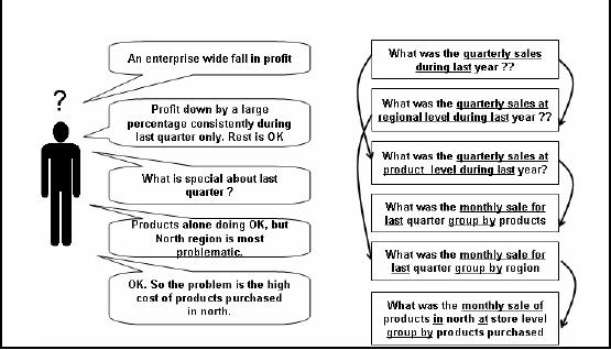
Figure -10.1. Consider a
hypothetical (but a realistic
scenario) when a
decision maker (analyst,
CEO) of a large enterprise
i.e. a multinational company
is confronted
with the yearly sales
figure that there is an
enterprise wide fall in
profit. Note that
we are talking
about a large multinational company,
which is not only in sales,
but also in
production. To
get a hold of the problem,
decision maker has to start
from somewhere, but
that
somewhere
has to be meaningful too.
This "somewhere" could be starting the
exploration across
the
enterprise geographically or exploring
across the enterprise
functionally or doing it product -
wise or
doing it with reference to
time.
One of
the valid options of starting is with
reference to time, and the query corresponding to
the
thought process
of the decision maker turns
out to be "What was the quarterly
sales during last
year?" The
result of this query would be sales
figures for the four
quarters of last year. There
can
be a number of
possible outcomes, for
example, the sale could be
down in all the quarters, or
it
could be down in
three out of four quarters
with four possible options.
Another possibility could
be sales
down in any two quarters
with six possible scenarios.
For the sake of simplicity,
over
here we
assume that the sales were
down in only one quarter. If
the results were displayed
as
histograms,
the decision maker would
immediately pick the quarter in which
sales were down,
which in
this case comes out to be
the last quarter.
Supporting
the human thought
process
THOUGHT
PROCESS
QUERY
SEQUENCE
Figure-10.1:
Supporting the human thought
process
61

Now
that the "lossy" quarter has
been identified, the
decision maker would naturally
like to probe
further, to go
to the root of the problem,
and would like to know what
happened during the
last
quarter that
resulted into a fall in
profit? The objective here
is to identify the root
cause, once
identified,
the problem can be fixed. So
the obvious question that
comes into the mind of
the
decision
maker is what is
special about the last
quarter? Before
jumping directly into the
last
quarter to come
up with hasty outcomes, the
careful decision maker wants
to look at the sales
data
of the
last year, but with a
different perspective, therefore, his/her
question is translated into
two
queries
i.e. (i) What was
the quarterly sales at regional level
during last year? (ii)
What was the
quarterly sal es
at product level during last
year? There could be another
sequence of questions
i.e.
probing
deeper into the "lossy" quarter directly,
which is followed in the
next sequence of
queries.
It may
seem that the decision
maker was overly careful,
but he was not. Recognize
that the
benefit of
looking at a whole year of
data enables the decision
maker to identify if there
was a
trend of sales
going down, that resulted in
least sales during the
last quarter or the sales
only went
down
during the last quarter? The
finding was that the
sales went down only
during the last
quarter, so
the decision maker probed
further by looking at the
sales at monthly basis during
the
last
quarter with reference to
product, as well as with
reference to region. Here is a finding,
the
sales were
doing all right with
reference to the product, but
they were found to be down
with
reference to
the region, specifically the Northern
region.
Now
the decision maker would
like to know what happened in
the Northern region in the
last
quarter
with reference to the
products, as just looking at
the Northern regional alone
would not
give
the complete picture. Although not
explicitly shown in the figure
-?, but the current
exploratory query of
the decision maker is
further processed by taking the
sales figures of last
quarter on
monthly basis and coupled
together with the product
purchased at store level.
Now the
hard work
pays off, as the problem has
finally been identified i.e.
high cost of products
purchased
during
the last quarter in the
Northe rn region. Well actually it
was not hard work in
its true literal
meaning, as
using an OLAP tool, this
would have taken not more
than a couple of
minutes,
maybe even
less.
Analysis of
last example
�
Analysis is
Ad-hoc
�
Analysis is
interactive (user driven)
�
Analysis is
iterative
� Answer to
one question leads to a
dozen more
�
Analysis is
directional
� Drill
Down
�
Roll
Up
�
Drill
Across
Now if we
carefully analyze the last
example, some points are
very clear, the first
one being
analysis is
ad-hoc i.e. there is no
known order to the sequence
of questions. The order of
the
questions
actually depends on the
outcome of the questions
asked, the domain knowledge of
the
decision
maker, and the inference
made by the decision maker
about the results
retrieved.
Furthermo re, it
is not possible to perform such an
analysis with a fixed set of
queries, as it is not
62

possible to
know in advance what questions
will be asked, and more
importantly what answers or
results
will be presented corresponding to those
questions. In a nut -shell, not
only the querying is
ad-hoc, but
the universal set of pre
-programmed queries is also
very large, hence it is a
very
complex
problem.
As you would
have experienced while using an
MIS system or done while
developing and MIS
system,
such systems are programmer
driven. One would disagree
with that, arguing
that
development
comes after system analysis,
when user has given his/her
requirements. The problem
with
decision support systems is
that, the user is unaware of
their requirements, until
they ha ve
used
the system. Furthermore, the number
and type of queries are
fixed as set by the
programmer,
thus if
the decision maker has to
use the OLTP system
for decision making, he is forced to
use
only
those queries that have
been pre-written thus the
process of decision making is driven not
by
the
decision maker. As we have seen,
the decision making is interactive i.e.
there is noting in
between
the decision support system
and the decision
maker.
In a traditional
MIS system, there is an
almost linear sequence of
queries i.e. one query
followed
by another,
with a limited number of queries to go
back to with almost fixed
and rigid results. As
a consequence,
running the same set of
queries in the same order
will not result in
something
new. As we
discussed in the example,
the decision support
processes is exploratory, and
depending on the
results obtained, the
queries are further fine
-tuned or the data is probed
deeply,
thus it is an
iterative process. Going
through the loop of queries
as per the requirement of the
decision
maker fine tunes the
results, as a result the
process actually results in coming up
with the
answers to
the questions.
Challenges
�
Not
feasible to write predefined
queries.
� Fails to
remain user_driven (becomes programmer
driven).
�
Fails to remain
ad_hoc and hence is not
interactive.
�
Enable
ad-hoc query support
� Business
user can not build his/her
own queries (does not know
SQL, should not
know
it).
�
On_the_go SQL
generation and execution too
slow.
Now
that we have identified how
decision making proceeds, this could
lure someone with an
OLTP or
MIS mindset to approach
decision support using the
traditional tools and
techniques.
Let's
look at this (wrong)
approach one point at a
time. We identified one very
important point
that
decision support requires
much more and many more
queries as compared to an MIS
system.
But even if more
queries are written, the
queries still remain predefined,
and the process of
decision making
still continues to be driven by
the programmer (who is not a decision
maker)
instead of
the decision maker. When
something is programmed, it kind of
gets hard-wired i.e.
it
can not be
changed significantly, although minor
changes are possible by changing
the parameter
values.
That's where the fault lies
i.e. hard -wiring. Decision
making has no particular order
associated
with it.
One could
naively say OK if the
decision making process has to be
user driven, let the end
user or
business
user do the query development himself/herself.
This is a very unrealistic assumption,
as
63

the
business user is not a programmer, does
not know SQL, and does not
need to know SQL. An
apparently
realistic solution would be to let the
SQL generation be on-the-go.
This approach does
make
the system user driven
without having the user to
write SQL, but even if on-the-go
SQL
generation can
be achieved, the data sets
used in a data warehouse are
so large, that it is no way
possible
for the system to remain
interactive!
Challenges
�
Contradiction
� Want to
compute answers in advance, but don't
know the questions
�
Solution
� Compute
answers to "all" possible "queries".
But how?
�
NOTE:
Queries are multidimensional aggregates
at some level
So what are
the challenges? We have a paradox or a
contradiction here. OK we manage
to
assemble a
very large team of dedicated
programmers, with an excellent project
manager and all
sit
and plan to write all
queries in advance. Can we do
that? The answer is a resounding
NO. The
reason being,
since even the user
dose not knows the queries
in advance, and consequently
the
programmers also
do not know the queries in
advance, so how can the
queries be written in
advance? It is
just no possible.
So what is the
solution then? We need a paradigm shift
from the way we have
been thinking. In a
decision
support environment, we are looking at
the big picture; we are
interested in all
sales
figures
across a time interval or at a particular time
interval, but not for a particular
person. So the
solution lies in
computing all possible aggregates,
which would then correspond
to all possible
queries.
Over here a query is a multidimensional
aggregate at a certain level of
the hierarchy of
the
business.
To understand
this concept, let's look at
Figure -10.2 that shows multiple levels
or hierarchies of
geographies.
Pakistan is logically divided
into provinces, and each
province is administratively
divided
into divisions, each division is
divided into districts and
within districts are
cities.
Consider a
chain store, with outlets in
major cities of Pakistan, with large
cities such as
Karachi
and Lahore
having multiple outlets,
which you may have observed
also. Now the sales
actually
take
place at the business outlet
which could be in a zone, such as
Defense and Gulberg in
our
example, of
course there may be many
more stores in a city, as
already discussed.
64
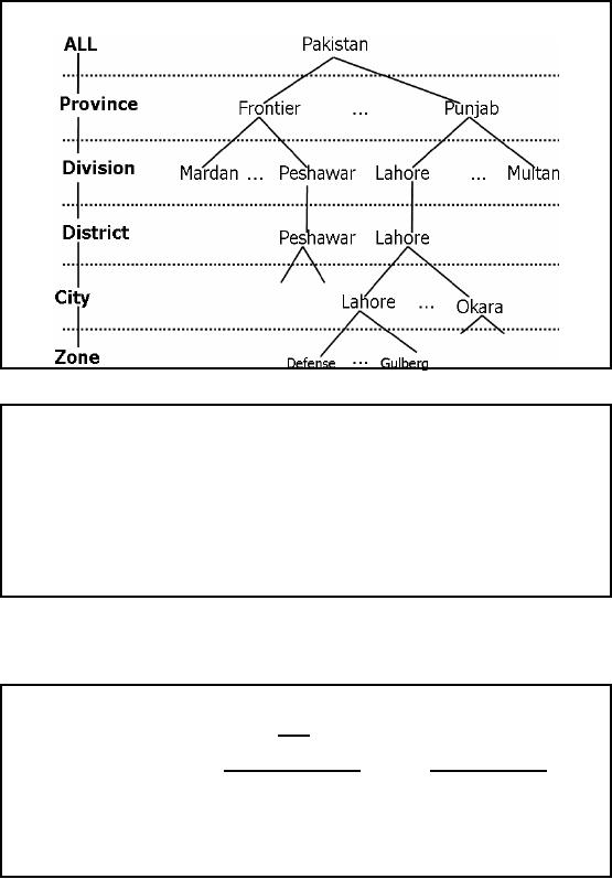
"All"
possible queries (level
aggregates)
Figure-10.2:
Hierarchies in data
OLAP:
Facts & Dimensions
�
FACTS:
Quantitative values (numbers) or
"measures."
� e.g.,
units sold, sales $, Co, Kg
etc.
�
DIMENSIONS:
Descriptive categories.
� e.g.,
time, geography, product
etc.
�
DIM
often organized in hierarchies
representing levels of detail in the data
(e.g.,
week,
month, quarter, year, decade
etc.).
The foundation
for design in this environment is through
use of dimensional modeling
techniques
which
focus on the concepts of
"facts" and "dimensions" for organizing
data. Facts are
the
quantities,
numbers that can be
aggregated (e.g., sales $,
units sold etc.) that we
measure and
dimensions
are how we filter/report on
the quantities (e.g., by
geography, product, date, etc.).
We
will
discuss in detail, actually
have number of lectures on dimensional modeling
techniques.
Where
Does OLAP Fit
In?
�
It is a
classification of applications, NOT a
database design
technique.
�
Analytical
processing uses multi-level
aggregates, instead of record level
access.
�
Objective is to
support very
�
(i)
fast
�
(ii) iterative
and
�
(iii)
ad-hoc decision-making.
65
OLAP is a
characterization of applications. It is
NOT a database design
technique. People
often
confuse
OLAP with specific physical
design techniques or data
structure. This is a
mistake.
OLAP is a
characterization of the application domain
centered around slice-and-dice and
drill
down
analysis. As we will see,
there are many possible
implementations capable of
delivering
OLAP
characteristics. Depending on data size,
performance requirements, cost
constraints, etc.
the specific
implementation technique will
vary.
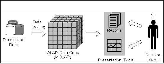
Where
does OLAP fit
in?
Figure-10.3:
How does OLAP pi eces
fir together
Figure -10.3
shows that using the
transactional databases (after
Extract Transform Load)
OLAP
data
cubes are generated. Over
here multidimensional cube is shown
i.e. a MOLAP cube.
Data
retrieved as a
consequence of exploring the
MOLAP cub e is then used as
a source to generate
reports or
charts etc. Actually in typical
MOLAP environments, the results
are displayed as
tables, along
with different types of
charts, such as histogram, pie
etc.
66
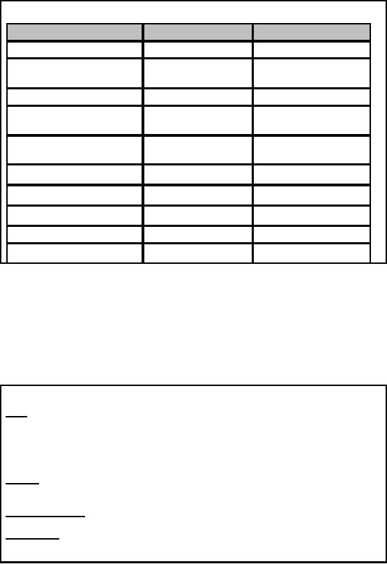
OLTP
vs. OLAP
Feature
OLTP
OLAP
Level of
data
Detailed
Aggregated
Amount of
data retrieved
per
Small
Large
transaction
Views
Pre-defined
User-defined
Typical
write operation
Update,
insert, delete
Bulk
insert, almost no
deletion
"age" of
data
Current (60-90
days)
Historical
5-10 years and
also
current
Tables
Flat
tables
Multi-Dimensional
tables
Number of
users
Large
Low-Med
Data
availability
High
(24 hrs, 7 days)
Low-Med
Database
size
Med
(GB- TB)
High
(TB PB)
Query
Optimizing
Requires
experience
Already
"optimized"
Table-10.1:
Difference between OLTP and
OLAP
The
table summarizes the fundamental
differences between traditional OLTP
systems and typical
OLAP
applications. In OLTP operations
the user changes the
database via transactions
on
detailed
data. A typical transaction in a banking environment
may transfer money from
one
account to
another account. In OLAP
applications the typical user is an
analyst who is
interested
in selecting
data needed for decision
support. He/She is primarily
not interested in detailed
dat a,
but usually in
aggregated data over large
sets of data as it gives the
big picture. A typical OLAP
query is to find
the average amount of money
drawn from ATM by those
customers who are
male,
and of age between 15 and 25
years from (say) Jinnah
Super Market Islamabad after 8
pm.
For
this kind of query there are
no DML operations and the
DBMS contents do not
change.
OLAP
FASMI Test
Fast:
Delivers
information to the user at a
fairly constant rate i.e.
O(1) time. Most
queries
answered in
under 5 seconds.
Analysis:
Performs
basic numerical and statistical
analysis of the data, pre -defined by
an
application developer or
defined ad-hocly by the
user.
Shared:
Implements
the security requirements
necessary for sharing potentially
confidential data
across a large
user population.
Multi-dimensional:
The
essential characteristic of
OLAP.
Information:
Accesses
all the data and
information necessary and
relevant for the
application,
wherever it
may reside and not
limited by volume.
67
FAST
means
that the system is targeted
to deliver response to moat of
the end user queries
under
5 seconds,
with the simplest analyses
taking no more than a second and
very few queries
taking
more than 20
seconds (for various reasons
to be discussed). Because if the
queries take
significantly
longer time, the thought
process is broken, as users are
likely to get
distracted,
consequently
the quality of analysis suffers.
This speed is not easy to
achieve with large amounts
of data,
particularly if on -the -go
and ad-hoc
complex
calculations are required.
ANALYSIS
means
that the system is capable
of doing any business logic
and statistical
analysis,
which is
applicable for the application and to
the user, and also
keeps it easy enough for
the user
i.e. at
the point -and-click level. It is
absolutely necessary to allow
the target user to define
and
execute
new ad hoc
calculations/queries
as part of the analysis and to
view the results of the
data
in any
desired way/format, without having to do
any programming.
SHARED
means
that the system is not
supposed to be a stand-alone system,
and should
implement all
the security requirements
for confidentiality (possibly
down to cell level) for
a
multi-user
environment. The other point is
kind of contradiction of the point
discussed earlier
i.e.
writing
back. If multiple DML
operations are needed to be performed,
concurrent update
locking
should be
executed at an appropriate level. It is
true that not all
applications require users to
write
data
back, but it is true for a
considerable majority.
MULTIDIMENSIONAL
is
the key requirement to the letter
and at the heart of the
cube concept
of OLAP.
The system must provide a
multidimensional logical view of the
aggregated data,
including
full support for hierarchies
and multiple hierarchies, as
this is certainly the most
logical
way to
analyze organizations and
businesses. There is no "magical" minimum
number of
dimensions
that must be handled as it is
too application specific.
INFORMATION
is
all of the data and
derived information required, wherever it
is and however
much is
relevant for the application.
The objective over here is
to ascertain the capacity of
various
products in
terms of how much input
data they can handle
and process, instead of how
many
Gigabytes of
raw data they can
store. There are many
considerations here, including
data
duplication,
Main Memory required, performance, disk
space utilization, integration with
data
warehouses
etc.
68
Table of Contents:
- Need of Data Warehousing
- Why a DWH, Warehousing
- The Basic Concept of Data Warehousing
- Classical SDLC and DWH SDLC, CLDS, Online Transaction Processing
- Types of Data Warehouses: Financial, Telecommunication, Insurance, Human Resource
- Normalization: Anomalies, 1NF, 2NF, INSERT, UPDATE, DELETE
- De-Normalization: Balance between Normalization and De-Normalization
- DeNormalization Techniques: Splitting Tables, Horizontal splitting, Vertical Splitting, Pre-Joining Tables, Adding Redundant Columns, Derived Attributes
- Issues of De-Normalization: Storage, Performance, Maintenance, Ease-of-use
- Online Analytical Processing OLAP: DWH and OLAP, OLTP
- OLAP Implementations: MOLAP, ROLAP, HOLAP, DOLAP
- ROLAP: Relational Database, ROLAP cube, Issues
- Dimensional Modeling DM: ER modeling, The Paradox, ER vs. DM,
- Process of Dimensional Modeling: Four Step: Choose Business Process, Grain, Facts, Dimensions
- Issues of Dimensional Modeling: Additive vs Non-Additive facts, Classification of Aggregation Functions
- Extract Transform Load ETL: ETL Cycle, Processing, Data Extraction, Data Transformation
- Issues of ETL: Diversity in source systems and platforms
- Issues of ETL: legacy data, Web scrapping, data quality, ETL vs ELT
- ETL Detail: Data Cleansing: data scrubbing, Dirty Data, Lexical Errors, Irregularities, Integrity Constraint Violation, Duplication
- Data Duplication Elimination and BSN Method: Record linkage, Merge, purge, Entity reconciliation, List washing and data cleansing
- Introduction to Data Quality Management: Intrinsic, Realistic, Orr’s Laws of Data Quality, TQM
- DQM: Quantifying Data Quality: Free-of-error, Completeness, Consistency, Ratios
- Total DQM: TDQM in a DWH, Data Quality Management Process
- Need for Speed: Parallelism: Scalability, Terminology, Parallelization OLTP Vs DSS
- Need for Speed: Hardware Techniques: Data Parallelism Concept
- Conventional Indexing Techniques: Concept, Goals, Dense Index, Sparse Index
- Special Indexing Techniques: Inverted, Bit map, Cluster, Join indexes
- Join Techniques: Nested loop, Sort Merge, Hash based join
- Data mining (DM): Knowledge Discovery in Databases KDD
- Data Mining: CLASSIFICATION, ESTIMATION, PREDICTION, CLUSTERING,
- Data Structures, types of Data Mining, Min-Max Distance, One-way, K-Means Clustering
- DWH Lifecycle: Data-Driven, Goal-Driven, User-Driven Methodologies
- DWH Implementation: Goal Driven Approach
- DWH Implementation: Goal Driven Approach
- DWH Life Cycle: Pitfalls, Mistakes, Tips
- Course Project
- Contents of Project Reports
- Case Study: Agri-Data Warehouse
- Web Warehousing: Drawbacks of traditional web sear ches, web search, Web traffic record: Log files
- Web Warehousing: Issues, Time-contiguous Log Entries, Transient Cookies, SSL, session ID Ping-pong, Persistent Cookies
- Data Transfer Service (DTS)
- Lab Data Set: Multi -Campus University
- Extracting Data Using Wizard
- Data Profiling