 |
Mapping Relationships, Binary, Unary Relationship, Data Manipulation Languages, Relational Algebra |
| << Database and Math Relations, Degree of a Relation |
| The Project Operator >> |

Database
Management System
(CS403)
VU
Lecture No.
16
Reading
Material
"Database
Systems Principles, Design
and Implementation"
Page
209
written
by Catherine Ricardo, Maxwell
Macmillan.
Overview of Lecture:
Mapping
Relationships
o
Binary
Relationships
o
Unary
Relationships
o
Data
Manipulation Languages
o
In the
previous lecture we discussed
the integrity constraints.
How conceptual
database
is converted into logical
database design, composite
and multi-valued
attributes.
In this lecture we will discuss
different mapping
relationships.
Mapping
Relationships
We have
up till now converted an
entity type and its
attributes into RDM.
Before
establishing
any relationship in between
different relations, it is must to study
the
cardinality
and degree of the relationship.
There is a difference in between
relation
and
relationship. Relation is a structure,
which is obtained by converting an
entity
type in
E-R model into a relation,
whereas a relationship is in between
two relations
of
relational data model.
Relationships in relational data model
are mapped according
to their
degree and cardinalities. It means
before establishing a relationship
there
cardinality
and degree is important.
Binary
Relationships
Binary
relationships are those,
which are established
between two entity
type.
Following
are the three types of
cardinalities for binary
relationships:
140

Database
Management System
(CS403)
VU
o One to
One
o One to
Many
o Many to
Many
In the
following treatment in each of
these situations is
discussed.
One to
Many:
In this
type of cardinality one instance of a
relation or entity type is
mapped with
many
instances of second entity type,
and inversely one instance of
second entity type
is mapped
with one instance of first
entity type. The
participating entity types will
be
transformed
into relations as has been
already discussed. The
relationship in this
particular
case will be implemented by placing
the PK of the entity type
(or
corresponding
relation) against one side
of relationship will be included in the
entity
type
(or corresponding relation) on
the many side of the
relationship as foreign
key
(FK). By
declaring the PK-FK link
between the two relations
the referential
integrity
constraint
is implemented automatically, which
means that value of foreign
key is
either
null or matches with its
value in the home
relation.
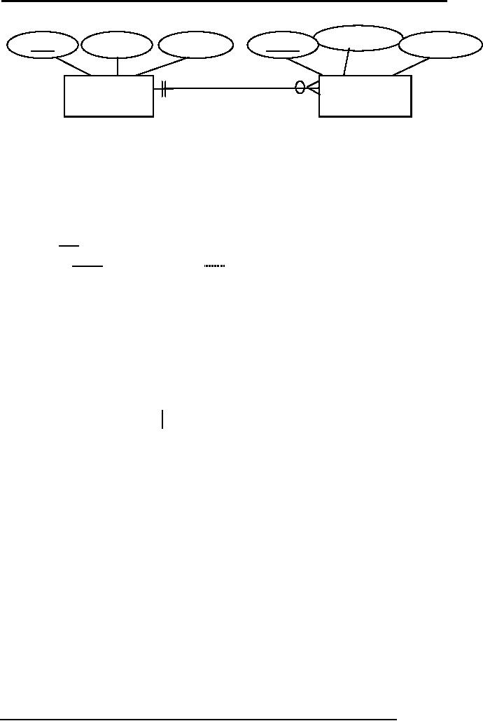
For
Example, consider the binary
relationship given in the
figure 1 involving
two
entity
types PROJET and EMPLOYEE.
Now there is a one to many
relationships
between
these two. On any one
project many employees can
work and one
employee
can
work on only one
project.
141
Database
Management System
(CS403)
VU
empNameme
prDuratio
prCost
empSal
prId
empId
np
PROJECT
EMPLOYEE
Fig. 1: A
one to many
relationship
The
two participating entity
types are transformed into
relations and the
relationship is
implemented
by including the PK of PROJECT
(prId) into the EMPLOYEE as
FK.
So the
transformation will be:
PROJECT
(prId, prDura,
prCost)
EMPLOYEE
(empId, empName, empSal,
prId)
The PK of
the PROJECT has been
included in EMPLOYEE as FK;
both keys do not
need to
have same name, but they
must have the same
domain.
Minimum
Cardinality:
This is a
very important point, as
minimum cardinality on one
side needs special
attention.
Like in previous example an
employee cannot exist if
project is not assigned.
So in
that case the minimum
cardinality has to be one. On
the other hand if an
instance of
EMPLOYEE can exist with
out being linked with an
instance of the
PROJECT
then the minimum cardinality
has to be zero. If the minimum
cardinality is
zero,
then the FK is defined as
normal and it can have
the Null value, on the
other
hand if
it is one then we have to
declare the FK attribute(s) as
Not Null. The Not
Null
constraint
makes it a must to enter the
value in the attribute(s) whereas
the FK
constraint
will enforce the value to be a
legal one. So you have to
see the minimum
cardinality
while implementing a one to
many relationship.
Many to Many
Relationship:
In this
type of relationship one instance of
first entity can be mapped
with many
instances
of second entity. Similarly
one instance of second entity
can be mapped
with
many instances of first
entity type. In many to many
relationship a third table
is
created
for the relationship, which
is also called as associative entity
type. Generally,
142

Database
Management System
(CS403)
VU
the
primary keys of the
participating entity types
are used as primary key of
the third
table.
For
Example, there are two
entity types BOOK and
STD (student). Now
many
students
can borrow a book and
similarly many books can be
issued to a student, so in
this
manner there is a many to
many relationship. Now there
would be a third
relation
as well
which will have its primary
key after combining primary
keys of BOOK and
STD. We
have named that as transaction
TRANS. Following are the
attributes of
these
relations: -
o STD
(stId, sName, sFname)
o BOOK
(bkId, bkTitle,
bkAuth)
o TRANS
(stId,bkId, isDate,rtDate)
Now here
the third relation TRANS
has four attributes first
two are the primary
keys
of two
entities whereas the last
two are issue date
and return date.
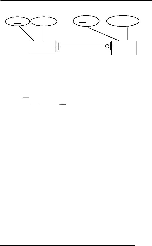
One to
One Relationship:
This is a
special form of one to many
relationship, in which one instance of
first entity
type is
mapped with one instance of
second entity type and
also the other way
round.
In this
relationship primary key of
one entity type has to be
included on other as
foreign
key. Normally primary key of
compulsory side is included in the
optional side.
For
example, there are two
entities STD and STAPPLE
(student application
for
scholarship).
Now the relationship from
STD to STAPPLE is optional
whereas
STAPPLE
to STD is compulsory. That
means every instance of
STAPPLE must be
related
with one instance of STD,
whereas it is not a must for an instance
of STD to
be
related to an instance of STAPPLE,
however, if it is related then it will be
related
to one
instance of STAPPLE, that is,
one student can give
just one scholarship
application.
This relationship is shown in
the figure below:
143
Database
Management System
(CS403)
VU
scAmount
scId
stName
stId
STD
SCAPPL
Fig. 2: A
one to one
relationship
While
transforming, two relations will be
created, one for STD and
HOBBY each. For
relationship
PK of either one can be
included in the other, it will
work. But preferably,
we should
include the PK of STD in
HOBBY as FK with Not Null
constraint imposed
on
it.
STD
(stId, stName)
STAPPLE
(scId, scAmount,
stId)
The
advantage of including the PK of
STD in STAPPLE as FK is that
any instance of
STAPPLE
will definitely have a value in
the FK attribute, that is,
stId. Whereas if we
do other
way round; we include the PK
of STAPPLE in STD as FK,
then since the
relationship
is optional from STD side,
the instances of STD may
have Null value in
the FK
attribute (scId), causing
the wastage of storage. More
the number records
with
Null
value more wastage.
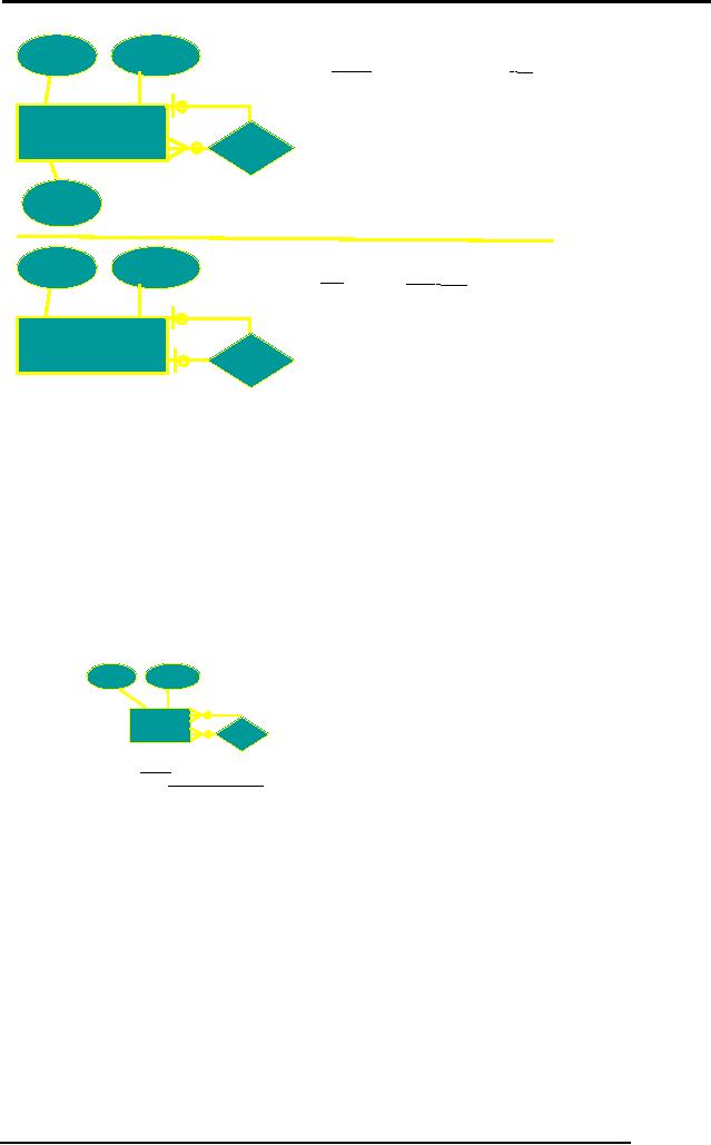
Unary
Relationship
These are
the relationships, which
involve a single entity.
These are also called
recursive
relationships. Unary relationships
may have one to one,
one to many and
many to
many cardinalities. In unary
one to one and one to
may relationships, the
PK
of same
entity type is used as
foreign key in the same
relation and obviously with
the
different
name since same attribute name
cannot be used in the same
table. The
example
of one to one relationship is
shown in the figure
below:
144
Database
Management System
(CS403)
VU
empId
empName
EMPLOYEE (empId,
empName, empAdr, mgr)
EMPLOYEE
MANAGES
empAdr
(a)
stId
stName
STUDENT (stId,
stName, roommate)
STUDENT
ROOMMATE
(b)
Fig. 3:
One to one relationships (a)
one to many (b) one to
one
and
their transformation
In many
to many relationships another
relation is created with composite
key. For
example
there is an entity type PART
may have many to many
recursive relationships,
meaning
one part consists of many
parts and one part may be
used in many parts. So
in this
case this is a many to many
relationship. The treatment of
such a relationship is
shown in
the figure below:
partId
partName
PART
MANAGES
PART
(partId, partName)
SUB-PART
(partId, component)
Fig. 4:
Recursive many to many
relationship
and
transformation
Super /
Subtype Relationship:
Separate
relations are created for
each super type and subtypes. It
means if there is
one
super type and there
are three subtypes, so then
four relations are to be
created.
After
creating these relations
then attributes are assigned.
Common attributes are
assigned
to super type and
specialized attributes are
assigned to concerned subtypes.
Primary
key of super type is included in
all relations that work
for both link
and
145

Database
Management System
(CS403)
VU
identity.
Now to link the super type
with concerned subtype there is a
requirement of
descriptive
attribute, which is called as
discriminator. It is used to identify
which
subtype
is to be linked. For Example
there is an entity type EMP
which is a super type,
now
there are three subtypes,
which are salaried, hourly
and consultants. So now
there
is a
requirement of a determinant, which
can identify that which
subtypes to be
consulted,
so with empId a special character
can be added which can be
used to
identify
the concerned subtype.
Summary
of Mapping E-R Diagram to
Relational DM:
We have
up till now studied that
how conceptual database
design is converted
into
logical
database. E-R data model is
semantically rich and it has
number of constructs
for
representing the whole
system. Conceptual database is
free of any data
model,
whereas
logical database the
required data model is chosen; in our
case it is relational
data
model. First we identified
the entity types, weak
and strong entity types.
Then we
converted
those entities into relations.
After converting entities
into relations then
attributes
are identified, different
types of attributes are identified.
Then relationships
were
made, in which cardinality and degree
was identified. In ternary
relationship,
where
three entities are involved,
in this as well another
relation is created to establish
relationship
among them. Then finally we
had studied the super and
sub types in
which
primary key of super type
was used for both
identity and link.
Data
Manipulation Languages
This is
the third component of
relational data model. We
have studied
structure,
which is
the relation, integrity
constraints both referential
and entity integrity
constraint.
Data manipulation languages are
used to carry out different
operations like
insertion,
deletion or creation of database.
Following are the two types
of languages:
146

Database
Management System
(CS403)
VU
Procedural
Languages:
These
are those languages in which what to do
and how to do on the
database is
required.
It means whatever operation is to be
done on the database that
has to be told
that
how to perform.
Non
-Procedural Languages:
These
are those languages in which only
what to do is required, rest
how to do is done
by the
manipulation language
itself.
Structured
query language (SQL) is the
most widely language used
for manipulation
of data.
But we will first study
Relational Algebra and
Relational Calculus, which
are
procedural
and non procedural
respectively.
Relational
Algebra
Following
are few major properties of
relational algebra:
o Relational
algebra operations work on one or
more relations to
define
another
relation leaving the
original intact. It means
that the input for
relational
algebra can be one or more
relations and the output
would be
another
relation, but the original
participating relations will
remain
unchanged
and intact.Both
operands and results are relations, so
output from
one
operation can become input to
another operation. It means
that the input
and
output both are relations so
they can be used iteratively
in different
requirements.
o Allows
expressions to be nested, just as in arithmetic.
This property is
called
closure.
o There
are five basic operations in
relational algebra: Selection,
Projection,
Cartesian
product, Union, and Set
Difference.
o These
perform most of the data retrieval
operations needed.
o It also
has Join, Intersection, and
Division operations, which
can be expressed
in terms
of 5 basic operations.
Exercise:
-
Consider
the example given in Ricardo
book on page 216 and
transform it into
relational
data model. Make any
necessary assumptions if required.
147
Table of Contents:
- Introduction to Databases and Traditional File Processing Systems
- Advantages, Cost, Importance, Levels, Users of Database Systems
- Database Architecture: Level, Schema, Model, Conceptual or Logical View:
- Internal or Physical View of Schema, Data Independence, Funct ions of DBMS
- Database Development Process, Tools, Data Flow Diagrams, Types of DFD
- Data Flow Diagram, Data Dictionary, Database Design, Data Model
- Entity-Relationship Data Model, Classification of entity types, Attributes
- Attributes, The Keys
- Relationships:Types of Relationships in databases
- Dependencies, Enhancements in E-R Data Model. Super-type and Subtypes
- Inheritance Is, Super types and Subtypes, Constraints, Completeness Constraint, Disjointness Constraint, Subtype Discriminator
- Steps in the Study of system
- Conceptual, Logical Database Design, Relationships and Cardinalities in between Entities
- Relational Data Model, Mathematical Relations, Database Relations
- Database and Math Relations, Degree of a Relation
- Mapping Relationships, Binary, Unary Relationship, Data Manipulation Languages, Relational Algebra
- The Project Operator
- Types of Joins: Theta Join, EquiJoin, Natural Join, Outer Join, Semi Join
- Functional Dependency, Inference Rules, Normal Forms
- Second, Third Normal Form, Boyce - Codd Normal Form, Higher Normal Forms
- Normalization Summary, Example, Physical Database Design
- Physical Database Design: DESIGNING FIELDS, CODING AND COMPRESSION TECHNIQUES
- Physical Record and De-normalization, Partitioning
- Vertical Partitioning, Replication, MS SQL Server
- Rules of SQL Format, Data Types in SQL Server
- Categories of SQL Commands,
- Alter Table Statement
- Select Statement, Attribute Allias
- Data Manipulation Language
- ORDER BY Clause, Functions in SQL, GROUP BY Clause, HAVING Clause, Cartesian Product
- Inner Join, Outer Join, Semi Join, Self Join, Subquery,
- Application Programs, User Interface, Forms, Tips for User Friendly Interface
- Designing Input Form, Arranging Form, Adding Command Buttons
- Data Storage Concepts, Physical Storage Media, Memory Hierarchy
- File Organizations: Hashing Algorithm, Collision Handling
- Hashing, Hash Functions, Hashed Access Characteristics, Mapping functions, Open addressing
- Index Classification
- Ordered, Dense, Sparse, Multi-Level Indices, Clustered, Non-clustered Indexes
- Views, Data Independence, Security, Vertical and Horizontal Subset of a Table
- Materialized View, Simple Views, Complex View, Dynamic Views
- Updating Multiple Tables, Transaction Management
- Transactions and Schedules, Concurrent Execution, Serializability, Lock-Based Concurrency Control, Deadlocks
- Incremental Log with Deferred, Immediate Updates, Concurrency Control
- Serial Execution, Serializability, Locking, Inconsistent Analysis
- Locking Idea, DeadLock Handling, Deadlock Resolution, Timestamping rules