Issues of De-Normalization: Storage, Performance, Maintenance, Ease-of-use

<< DeNormalization Techniques: Splitting Tables, Horizontal splitting, Vertical Splitting, Pre-Joining Tables, Adding Redundant Columns, Derived Attributes

Online Analytical Processing OLAP: DWH and OLAP, OLTP >>

Lecture Handout

Data Warehousing

Lecture No. 09

Issues of De-Normalization

Storage

Performance

Maintenance

Ease-of-use

The effects of denormalization on database performance are unpredictable: as many

applications/users can be affected negatively by denormalization when some applications are

optimized. If a decision is made to denormalize, make sure that the logical model has been fully

normalized to 3NF. Also document the pure logical model and keep your documentation of the

physical model current as well. Consider the following list of effects of denormalization before

you decide to undertake design changes.

The trade-offs of denormalization are as follows:

Storage

Performance

Ease-of-use

Maintenance

Each of these tradeoffs must be considered when deploying denormalization into a physical

design. Typically, architects are pretty good at assessing performance and storage implications of

a denormalization decision. Factors that are notoriously under estimated are the maintenance

implications and the impact on usability/flexibility for the physical data model.

Storage Issues: Pre-joining

Assume 1:2 record count ratio between claim master and detail for health-care

application.

Assume 10 million members (20 million records in claim detail).

Assume 10 byte member_ID.

Assume 40 byte header for master and 60 byte header for detail tables.

By understanding the characteristics of the data, the storage requirements can actually be

quantified before pre -joining. We need to know the size of the data from the master table that

will be replicated for pre -joining into the detail table as well as the number of detail records (on

average) in the header that will be denormalized as a result of pre -joining.

In this example, it is assumed that that each master table record has two detail record entries

associated with it (on average). Note that this ratio will vary depending on the nature of each

industry and business within an industry. The health-care industry would be much closer to a 1:2

ratio, depending on if the data is biased towards individual or organizational claims. A 1:3 ratio

could be reasonable for a video rental store, but a grocery store with tens of thousands of items,

the ratio would typically be on the plus side of 1:30 detail records for each master table entry. It is

important to know the characteristics in your specific environment to properly and correctly

calculate the storage requirements of the pre -joining technique.

Storage Issues: Pre-joining

With normalization:

Total space used = 10 x 40 + 20 x 60 = 1.6 GB

After denormalization:

Total space used = (60 + 40 10) x 20 = 1.8 GB

Net result is 12.5% additional space required in raw data table size for the database.

The 12.5% investment in additional storage for pre -joining will dramatically increase

performance for queries which would otherwise need to join the very large header and detail

tables.

Performance Issues: Pre-joining

Consider the query "How many members were paid claims during last year?"

With normalization:

Simply count the number of records in the master table.

After denormalization:

The member_ID would be repeated, hence need a count distinct. This will cause sorting

on a larger table and degraded performance.

How the corresponding query will perform with normalization and after denormalization? This a

good question, with a surprising answer. Observe that with normalization there are unique values

in the master table, and the number of records in the master table is the required answer. To get

this answer, there is probably no need to touch that table, as the said information can be picked

from the meta-data corresponding to that table. However, it is a different situ tion after pre -

joining has been performed. Now there are multiple i.e. repeating member_IDs in the joined

table. Thus accessing the meta-data is not going to help. The only viable option is to perform a

count distinct, easier said than done. The reason be ing this will require a sort operation, and then

dropping the repeating value. For large tables, it is going to kill the performance of the system.

Performance Issues: Pre-joining

Depending on the query, the performance actually deteriorates with denorma lization! This is due

to the following three reasons:

Forcing a sort due to count distinct.

Using a table with 2.5 times header size.

Using a table which is 2 times larger.

Resulting in 5 times degradation in performance.

Bottom Line: Other than 0.2 GB additional space, also keep the 0.4 GB master table.

Counter intuitively, the query with pre -joining will perform worse than the normalized design,

basically for three reasons.

1. There is no simple way to count the number of distinct customers in t he physical data

model because this information is now "lost" in the detail table. As a result, there is no

choice, but to use a "count distinct" on the member_ID to group identical IDs and then

determine the number of unique patients. This is going to be achieved by sorting all

qualifying rows (by date) in the denormalized tables. Note that sorting is typically a very

expensive operation, the best being O(n log n).

2. The table header of the denormalized detail table is now 90 bytes as opposed to 40 bytes

of the master table i.e. an increase of 250%.

3. The number of rows that need to be scanned in the details table are two times as many as

compared to the normalized design i.e. scanning the master table. This translates to five

times more I/Os in the denormalized scenario versus the normalized scenario!

Bottom line is that the normalized design is likely to perform many times faster as compared to

the denormalized design for queries that probe the master table alone, rather than those that

perform a join bet ween the master and the detail table. Best and expensive approach would be to

also keep the normalized master table, and a smart query coordinator that directs the queries to

for increasing performance.

Performance Issues: Adding redundant columns

Continuing with the previous Health-Care example, assuming a 60 byte detail table and 10 byte

Sale_Person.

Copying the Sale_Person to the detail table results in all scans taking 16% longer

than previously.

Justifiable only if significant portion of queries get benefit by accessing the

denormalized detail table.

Need to look at the cost-benefit trade-off for each denormalization decision.

The main problem with redundant columns is that if strict discipline is not enforced, it can very

quickly result into chaos. The reason being, every DWH user has their own set of columns which

they frequently use in their queries. Once they hear about the performance benefits (due to

denormalization) they would want their "favorite" column(s) to be moved/copied into the main

fact table in the data warehouse. If this is allowed to happen, sooner than later the fact table

would become one large flat file with a header in kilo bytes, and result in degraded performance.

The reason being, each time the table width is increased, the number of rows per block decreases

and the amount of I/O increases, and the table access becomes less efficient. Hence the column

redundancy can not be looked into isolation, with a view to benefit a only a subset of the queries.

For a number of queries, the performance will degrade by avoiding the join, thus a detailed and

quantifiable cost-benefit analysis is required.

Other Issues: Adding redundant columns

Other issues include, increase in table size, maintenance and loss of information:

The size of the (largest table i.e.) transaction table increases by the size of the

Sale_Person key.

§ For the example being considered, the detail table size increases from 1.2 GB to

1.32 GB.

If the Sale_Person key changes (e.g. new 12 digit NID), then updates to be reflected all

the way to transaction table.

In the absence of 1:M relationship, column movement will actually result in loss of data.

Maintenance is usually overlooked or underestimated while replicating columns. Because the cost

of reflecting the change in the member_ID for this design, is considerably high when reflected

across the relevant tables. For example, transactions in the detail table need to be updated with the

new key, and for a retail warehouse, the detail table could be 30 times larger than the master

table, which again is larger then the fact (member table). For an archival system that keeps

backup of the historical transactions, maintenance becomes a nightmare, because keeping the

member_id data consistent will be very risky.

Ease of use Issues: Horizontal Splitting

Horizontal splitting is a Divide&Conquer technique that exploits parallelism. The conquer part of

the technique is about combining the results.

Lets see how it works for hash based splitting/partitioning.

Assu ming uniform hashing, hash splitting supports even data distribution across all

partitions in a pre -defined manner.

However, hash based splitting is not easily reversible to eliminate the split.

Hash partitioning is the most common partitioning strategy. Almost all parallel RDBMS

products provide some form of built-in hash partitioning capability (mainframe DB2 is the most

significant exception to this statement). Horizontal partitioning using a hashing algorithm will

assign data rows to partitions according to a "repeatable" random algorithm. In other words, a

particular row will always hash to the same partition (assuming that the hashing algorithm and

number of partitions have not changed), but a large number of rows will be "randomly"

distributed across the partitions as long as a well-selected partitioning key is selected and the

hashing function is well-behaved.

Notice that the "random" assignment of data rows across partitions makes it nearly impossible to

get any kind of meaningful partition elimination. Since data rows are hash distributed across all

partitions (for load-balancing purposes), there is not practical way to perform partition

elimination unless a very small number (e.g., singleton) or data rows is selected from the table via

the partitioning key (which doesn't happen often in a traditional DW workload).

Ease of Use Issues: Horizontal Splitting

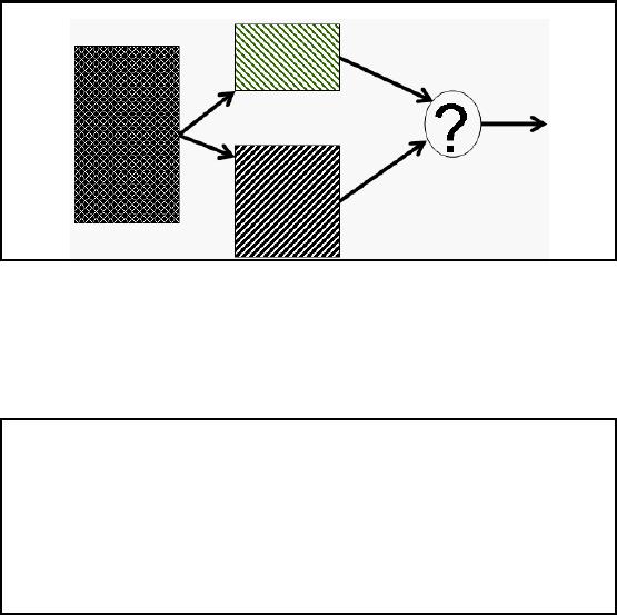
Figure-9.1: Irreversible partitioning

Note that we perform denormalization to get performance for a particular set of queries, and may

like to bring the table back to its original form for another set of queries. If this can not be done,

then extra effort or CPU cycles would be required to achieve this objective. As shown in Figure -

9.1, it is possible to have a part itioning strategy, such that the partitioned tables can not be

appended together to get the record sin the original order. This is further explained when we

discuss the issues of horizontal partitioning.

Ease of Use Issues: Horizontal Splitting

Round robin and random splitting:

§ Guarantee good data distribution.

§ Not pre-defined.

§ Almost impossible to reverse (or undo).

Range and expression splitting:

§ Can facilitate partition elimination with a smart optimizer.

§ Generally lead to "hot spots" (uneven distribution of data).

Round-robin spreads data evenly across the partitions, but does not facilitate partition elimination

(for the same reasons that hashing does not facilitate partition elimination). Round -robin is

typically used only for temporary tables where partition elimination is not important and co -

location of the table with other tables is not expected to yield performance benefits (hashing

allows for co-location, but round-robin does not). Round -robin is the "cheapest" partitioning

algorithm that guarantees an even distribution of workload across the table partitions.

The most common use of range partitioning is on date. This is especially true in data warehouse

deployments where large amounts of historical data are often retained. Hot spots typically

surface when using date range partitioning because the most recent data tends to be accessed most

frequently.

Expression partitioning is usually deployed when expressions can be used to group data together

in such a way that access can be targeted to a small set of partitions for a significant portion of the

DW workload. For example, partitioning a table by expression so that data corresponding to

different divisions or LOBs (lines of business) is grouped together will avoid scanning data in

divisions or LOBs excluded from the WHERE clause predicates in a DSS query. Expression

partitioning can lead to hot spots in the same way as described for range partitioning.

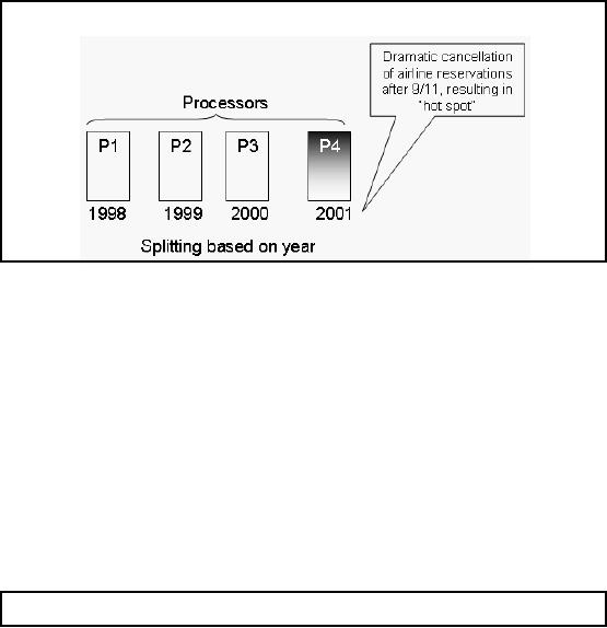
Performance Issues: Horizontal Splitting

Figure-9.2: De-mertis of horizontal partitoiniong

Recall in last lecture when we discussed partitioning on the basis of date to enhance query

performance, this has its down sides too. Consider the case of airline reservations table

horizontally split on the basis of year. After 9/11 people obviously got scared of flying, and there

was a surge of cancellations of air line bookings. Thus the most number of cancellations, actually,

probably highest ever occurred during the last quarter of year 2001. Thus the corresponding

part ition would have the largest number of records. Thus in a parallel processing environment,

where partitioning is consciously done to improve performance it not going to work, because as

shown in Figure-9.2 most of the work is being done by processor P4 which would become a

bottleneck. Meaning, unless the results of processor P4 are made available, the overall results can

not be combined, while the remaining processors are idling i.e. doing nothing.

Performance issues: Vertical Splitting

Example: Consider a 100 byte header for the member table such that 20 bytes provide complete

coverage for 90% of the queries.

Split the member table into two parts as follows:

1. Frequently accessed portion of table (20 bytes), and

2. Infrequently accessed portion of table (80+ bytes). Why 80+?

Note that primary key (member_id) must be present in both tables for eliminating the split.

Note that there will be a one-to-one relationship between rows in the two portions of the

partitioned table.

Performance issues: Vertical Splitting

Scanning the claim table for most frequently used queries will be 500% faster with vertical

splitting

Ironically, for the "infrequently" accessed queries the performance will be inferior as compared to

the un -split table because of the join overhead.

Scanning the vertically partitioned claim table for frequently accessed data is five times faster

than before splitting because the table is five times "thinner" without the infrequently used

portions of the data.

However, this performance benefit will only be obtained if we do not have to join to the

infrequently accessed portion of the table. In other words, all columns that we need must be in

the frequently accessed portion of the table.

Performance issues: Vertical Splitti ng

Carefully identify and select the columns that get placed on which "side" of the

frequently/infrequently used "divide" between the splits.

Moving a single five byte column to the frequently used table split (20 byte width) means that

ALL table scans a gainst the frequently used table will run 25% slower.

Don't forget the additional space required for the join key, this becomes significant for a billion

row table.

Also, be careful when determining frequency of use. You may have 90% of the queries accessing

columns in the "frequently used" partition of the table. However, the important measure is the

percent of queries that access only the frequently used portion of the table with no columns

required from the infrequently used data.

Table of Contents: