 |

Database
Management System
(CS403)
VU
Lecture No.
15
Reading
Material
Overview of
Lecture
Database
and Math Relations
o
Degree
and Cardinality of
Relation
o
Integrity
Constraints
o
Transforming
conceptual database design
into logical database
design
o
Composite
and multi-valued
Attributes
o
Identifier
Dependency
o
In the
previous lecture we discussed
relational data model, its
components and
properties
of a table. We also discussed
mathematical and database
relations. Now we
will
discuss the difference in
between database and
mathematical relations.
Database
and Math Relations
We
studied six basic properties of tables or
database relations. If we compare
these
properties
with those of mathematical relations
then we find out that
properties of
both
are the same except
the one related to order of
the columns. The order
of
columns
in mathematical relations does
matter, whereas in database
relations it does
not
matter. There will not be
any change in either math or
database relations if we
change
the rows or tuples of any
relation. It means that the
only difference in
between
these
two is of order of columns or
attributes. A math relation is a
Cartesian product
of two
sets. So if we change the order of
theses two sets then
the outcome of both
will
not be
same. Therefore, the math
relation changes by changing
the order of columns.
For
Example , if there is a set A
and a set B if we take
Cartesian product of A and
B
then we
take Cartesian product of B
and A they will not be equal
, so
AxB=BxA
Rests of
the properties between them
are same.
132

Database
Management System
(CS403)
VU
Degree of
a Relation
We will
now discuss the degree of a
relation not to be confused
with the degree of a
relationship.
You would be definitely
remembering that the
relationship is a link or
association
between one or more entity
types and we discussed it in
E-R data model.
However
the degree of a relation is the
number of columns in that
relation. For
Example
consider the table given
below:
STUDENT
StID
stName
clName
Sex
S001
Suhail
MCS
M
S002
Shahid
BCS
M
S003
Naila
MCS
F
S004
Rubab
MBA
F
S005
Ehsan
BBA
M
Table 1:
The STUDENT table
Now in
this example the relation
STUDENT has four columns, so
this relation has
degree
four.
Cardinality
of a Relation
The
number of rows present in a relation is
called as cardinality of that
relation. For
example,
in STUDENT table above, the
number of rows is five, so
the cardinality of
the
relation is five.
Relation
Keys
The
concept of key and all
different types of keys is
applicable to relations as
well.
We will
now discuss the concept of
foreign key in detail, which
will be used quite
frequently
in the RDM.
Foreign
Key
An
attribute of a table B that is
primary key in another table
A is called as foreign
key.
For
Example, consider the
following two tables EMP
and DEPT:
EMP
(empId, empName, qual,
depId)
DEPT
(depId, depName,
numEmp)
In this
example there are two
relations; EMP is having
record of employees,
whereas
DEPT is
having record of different departments of
an organization. Now in EMP
the
primary
key is empId, whereas in DEPT
the primary key is depId.
The depId which is
primary
key of DEPT is also present in EMP so
this is a foreign
key.
Requirements/Constraints
of Foreign Key
Following
are some requirements /
constraints of foreign
key:
There
can be more than zero, one
or multiple foreign keys in a
table, depending on
how
many tables a particular
table is related with. For
example in the above
example
the
EMP table is related with
the DEPT table, so there is
one foreign key
depId,
133

Database
Management System
(CS403)
VU
whereas
DEPT table does not
contain any foreign key.
Similarly, the EMP table
may
also be
linked with DESIG table
storing designations, in that
case EMP will have
another
foreign key and
alike.
The
foreign key attribute, which
is present as a primary key in another
relation is
called as
home relation of foreign key
attribute, so in EMP table
the depId is foreign
key
and its home relation is
DEPT.
The
foreign key attribute and
the one present in another
relation as primary key
can
have
different names, but both
must have same domains. In
DEPT, EMP example,
both
the PK and FK have the
same name; they could have
been different, it would
not
have
made any difference however
they must have the same
domain.
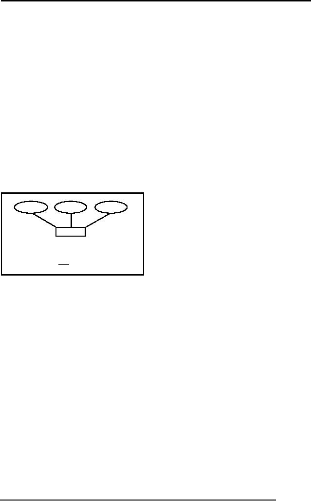
The
primary key is represented by underlining
with a solid line, whereas
foreign key
is
underlined by dashed or dotted
line.
Primary
Key :
Foreign
Key :
Integrity
Constraints
Integrity
constraints are very
important and they play a
vital role in relational
data
model.
They are one of the three
components of relational data model.
These
constraints
are basic form of constraints, so basic
that they are a part of the
data model,
due to
this fact every DBMS
that is based on the RDM must
support them.
Entity
Integrity Constraint:
It states
that in a relation no attribute of a
primary key (PK) can
have null value. If a
PK
consists of single attribute,
this constraint obviously
applies on this attribute, so
it
cannot
have the Null value.
However, if a PK consists of multiple
attributes, then
none of
the attributes of this PK
can have the Null
value in any of the
instances.
Referential
Integrity Constraint:
This
constraint is applied to foreign
keys. Foreign key is an
attribute or attribute
combination
of a relation that is the
primary key of another
relation. This
constraint
states
that if a foreign key exists
in a relation, either the
foreign key value must
match
the
primary key value of some
tuple in its home relation
or the foreign key value
must
be
completely null.
Significance
of Constraints:
By
definition a PK is a minimal identifier
that is used to identify
tuples uniquely. This
means
that no subset of the
primary key is sufficient to
provide unique
identification
of
tuples. If we were to allow a
null value for any
part of the primary key, we
would
be
demonstrating that not all
of the attributes are needed to
distinguish between
tuples,
which
would contradict the
definition.
Referential
integrity constraint plays a
vital role in maintaining
the correctness,
validity
or integrity of the database.
This means that when we
have to ensure the
proper
enforcement of the referential
integrity constraint to ensure
the consistency and
correctness
of database. How? In the
DEPT, EMP example above
deptId in EMP is
foreign
key; this is being used as a
link between the two
tables. Now in every
instance
of EMP
table the attribute deptId
will have a value, this
value will be used to get
the
name
and other details of the
department in which a particular
employee works. If
the
value of
deptId in EMP is Null in a
row or tuple, it means this
particular row is not
related
with any instance of the
DEPT. From real-world scenario it
means that this
particular
employee (whose is being represented by
this row/tuple) has not
been
134

Database
Management System
(CS403)
VU
assigned
any department or his/her
department has not been
specified. These were
two
possible conditions that are
being reflected by a legal
value or Null value of
the
foreign
key attribute. Now consider
the situation when
referential integrity constrains
is being
violated, that is,
EMP.deptId contains a value
that does not match with
any of
the
value of DEPT.deptId. In this
situation, if we want to know
the department of an
employee,
then ooops, there is no
department with this Id,
that means, an
employee
has been
assigned a department that does
not exist in the
organization or an illegal
department.
A wrong situation, not
wanted. This is the
significance of the
integrity
constraints.
Null
Constraints:
A Null
value of an attribute means
that the value of attribute
is not yet given,
not
defined
yet. It can be assigned or
defined later however.
Through Null constraint
we
can
monitor whether an attribute
can have Null value or
not. This is important and
we
have to
make careful use of this
constraint. This constraint is
included in the
definition
of a table (or an attribute
more precisely). By default a
non-key attribute
can
have Null value, however, if
we declare an attribute as Not
Null, then this
attribute
must be assigned value while entering a
record/tuple into the table
containing
that
attribute. The question is,
how do we apply or when do we
apply this
constraint,
or why
and when, on what basis we
declare an attribute Null or
Not Null. The answer
is,
from the system for
which we are developing the
database; it is generally an
organizational
constraint. For example, in a
bank, a potential customer has to fill in
a
form
that may comprise of many
entries, but some of them
would be necessary to fill
in,
like, the residential
address, or the national Id card
number. There may be
some
entries
that may be optional, like
fax number. When defining a
database system for
such a
bank, if we create a CLIENT
table then we will declare
the must attributes as
Not
Null, so that a record
cannot be successfully entered
into the table until at
least
those
attributes are not
specified.
Default
Value:
This
constraint means that if we do
not give any value to
any particular attribute,
it
will be
given a certain (default)
value. This constraint is
generally used for
the
efficiency
purpose in the data entry process.
Sometimes an attribute has a
certain
value
that is assigned to it in most of the
cases. For example, while
entering data for
the
students, one attribute holds
the current semester of the
student. The value of
this
attribute
is changed as a students passes through
different exams or semesters
during
its
degree. However, when a student is
registered for the first
time, it is generally
registered
in the first semesters. So in
the new records the value of
current semester
attribute
is generally 1. Rather than
expecting the person entering
the data to enter 1
in
every
record, we can place a
default value of 1 for this
attribute. So the person
can
simply
skip the attribute and
the attribute will automatically
assume its default
value.
Domain
Constraint:
This is
an essential constraint that is applied
on every attribute, that is,
every attribute
has
got a domain. Domain means
the possible set of values
that an attribute can
have.
For
example, some attributes may
have numeric values, like
salary, age, marks
etc.
Some
attributes may possess text
or character values, like, name
and address. Yet
some
others may have the date
type value, like date of
birth, joining date.
Domain
specification
limits an attribute the
nature of values that it can
have. Domain is
specified
by associating a data type to an
attribute while defining it.
Exact data type
name or
specification depends on the particular
tool that is being used.
Domain helps
135

Database
Management System
(CS403)
VU
to
maintain the integrity of
the data by allowing only
legal type of values to
an
attribute.
For example, if the age
attribute has been assigned a
numeric data type
then
it will
not be possible to assign a
text or date value to it. As a
database designer, this
is
your
job to assign an appropriate
data type to an attribute.
Another perspective
that
needs to
be considered is that the
value assigned to attributes
should be stored
efficiently.
That is, domain should
not allocate unnecessary
large space for
the
attribute.
For example, age has to be
numeric, but then there are
different types of
numeric
data types supported by different
tools that permit different
range of values
and
hence require different storage
space. Some of more
frequently supported
numeric
data types include Byte,
Integer, and Long Integer.
Each of these types
supports
different range of numeric values
and takes 1, 4 or 8 bytes to store. Now,
if
we
declare the age attribute as
Long Integer, it will definitely serve
the purpose, but
we will be
allocating unnecessarily large
space for each attribute. A
Byte type would
have been
sufficient for this purpose since
you won't find students or
employees of
age
more than 255, the
upper limit supported by
Byte data type. Rather we
can further
restrict
the domain of an attribute by
applying a check constraint on the
attribute. For
example,
the age attribute although
assigned type Byte, still if a person by
mistake
enters
the age of a student as 200,
if this is year then it is
not a legal age from
today's
age,
yet it is legal from the
domain constraint perspective. So we
can limit the
range
supported
by a domain by applying the check
constraint by limiting it up to say 30
or
40,
whatever is the rule of the
organization. At the same
time, don't be too
sensitive
about
storage efficiency, since attribute
domains should be large
enough to cater the
future
enhancement in the possible set of
values. So domain should be a
bit larger
than
that is required today. In
short, domain is also a very
useful constraint and
we
should
use it carefully as per the
situation and requirements in
the organization.
RDM
Components
We have
up till now studied
following two components of
the RDM, which are
the
Structure
and Entity Integrity
Constraints. The third part,
that is, the
Manipulation
Language
will be discussed in length in the
coming lectures.
Designing
Logical Database
Logical
data base design is obtained
from conceptual database
design. We have seen
that
initially we studied the
whole system through
different means. Then we
identified
different
entities, their attributes
and relationship in between
them. Then with the
help
of E-R
data model we achieved an E-R
diagram through different
tools available in
this
model. This model is
semantically rich. This is
our conceptual database
design.
Then as
we had to use relational data
model so then we came to
implementation phase
for
designing logical database
through relational data
model.
The
process of converting conceptual
database into logical
database involves
transformation
of E-R data model into
relational data model. We have
studied both
the data
models, now we will see how
to perform this
transformation.
Transforming
Rules
Following
are the transforming rules
for converting conceptual
database into logical
database
design:
The
rules are straightforward ,
which means that we just
have to follow the
rules
mentioned
and the required logical
database design would be
achieved
136
Database
Management System
(CS403)
VU
There
are two ways of transforming
first one is manually that
is we analyze and
evaluate
and then transform. Second is
that we have CASE tools
available with us
which
can automatically convert
conceptual database into
required logical
database
design
If we are
using CASE tools for
transforming then we must evaluate it as
there are
multiple
options available and we must
make necessary changes if
required.
Mapping
Entity Types
Following
are the rules for
mapping entity types:
Each
regular entity type (ET) is
transformed straightaway into a
relation. It means
that
whatever
entities we had identified
they would simply be
converted into a relation
and
will have
the same name of relation as
kept earlier.
Primary
key of the entity is
declared as Primary key of
relation and
underlined.
Simple
attributes of ET are included
into the relation
For
Example, figure 1 below
shows the conversion of a
strong entity type
into
equivalent
relation:
stName
stDoB
stId
STUDENT
STUDENT
(stId, stName, stDoB)
Fig. 1: An
example strong entity
type
Composite
Attributes
These
are those attributes which
are a combination of two or
more than two
attributes.
For
address can be a composite
attribute as it can have
house no, street no, city
code
and
country , similarly name can be a
combination of first and
last names. Now in
relational
data model composite attributes
are treated differently.
Since tables can
contain
only atomic values composite
attributes need to be represented as a
separate
relation
For
Example in student entity
type there is a composite
attribute Address, now in
E-R
model it
can be represented with simple
attributes but here in relational data
model,
there is
a requirement of another relation
like following:
137

Database
Management System
(CS403)
VU
stName
stDoB
stId
houseNo
STUDENT
streetNo
stAdres
country
areaCode
city
cityCode
STUDENT
(stId, stName, stDoB)
STDADRES
(stId, hNo, strNo, country,
cityCode, city,
areaCode)
Fig. 2:
Transformation of composite
attribute
Figure 2
above presents an example of
transforming a composite attribute
into RDM,
where it
is transformed into a table
that is linked with the
STUDENT table with
the
primary
key
Multi-valued
Attributes
These
are those attributes which
can have more than
one value against an
attribute.
For
Example a student can have
more than one hobby
like riding, reading
listening to
music
etc. So these attributes are
treated differently in relational data
model.
Following
are the rules for
multi-valued attributes:-
An Entity
type with a multi-valued
attribute is transformed into
two relations
One
contains the entity type
and other simple attributes
whereas the second one
has
the
multi-valued attribute. In this
way only single atomic
value is stored against
every
attribute
The
Primary key of the second
relation is the primary key
of first relation and
the
attribute
value itself. So in the
second relation the primary
key is the combination
of
two
attributes.
138

Database
Management System
(CS403)
VU
All
values are accessed through
reference of the primary key
that also serves as
stName
stDoB
stId
houseNo
STUDENT
streetNo
stHobby
stAdres
country
areaCode
city
cityCode
STUDENT (stId,
stName, stDoB)
STDADRES (stId,
hNo, strNo, country, cityCode,
city, areaCode)
STHOBBY(stId,
stHobby)
Fig. 3:
Transformation of multi-valued
attribute
foreign
key.
Conclusion
In this
lecture we have studied the
difference between mathematical
and database
relations.
The concepts of foreign key
and especially the integrity
constraints are very
important
and are basic for every
database. Then how a
conceptual database is
transformed
into logical database and in
our case it is relational data
model as it is the
most
widely used. We have also
studied certain transforming
rules for converting
E-R
data
model into relational data
model. Some other rule for
this transformation will be
studied
in the coming
lectures
You will
receive exercise at the end of
this topic.
139
Table of Contents:
- Introduction to Databases and Traditional File Processing Systems
- Advantages, Cost, Importance, Levels, Users of Database Systems
- Database Architecture: Level, Schema, Model, Conceptual or Logical View:
- Internal or Physical View of Schema, Data Independence, Funct ions of DBMS
- Database Development Process, Tools, Data Flow Diagrams, Types of DFD
- Data Flow Diagram, Data Dictionary, Database Design, Data Model
- Entity-Relationship Data Model, Classification of entity types, Attributes
- Attributes, The Keys
- Relationships:Types of Relationships in databases
- Dependencies, Enhancements in E-R Data Model. Super-type and Subtypes
- Inheritance Is, Super types and Subtypes, Constraints, Completeness Constraint, Disjointness Constraint, Subtype Discriminator
- Steps in the Study of system
- Conceptual, Logical Database Design, Relationships and Cardinalities in between Entities
- Relational Data Model, Mathematical Relations, Database Relations
- Database and Math Relations, Degree of a Relation
- Mapping Relationships, Binary, Unary Relationship, Data Manipulation Languages, Relational Algebra
- The Project Operator
- Types of Joins: Theta Join, Equi–Join, Natural Join, Outer Join, Semi Join
- Functional Dependency, Inference Rules, Normal Forms
- Second, Third Normal Form, Boyce - Codd Normal Form, Higher Normal Forms
- Normalization Summary, Example, Physical Database Design
- Physical Database Design: DESIGNING FIELDS, CODING AND COMPRESSION TECHNIQUES
- Physical Record and De-normalization, Partitioning
- Vertical Partitioning, Replication, MS SQL Server
- Rules of SQL Format, Data Types in SQL Server
- Categories of SQL Commands,
- Alter Table Statement
- Select Statement, Attribute Allias
- Data Manipulation Language
- ORDER BY Clause, Functions in SQL, GROUP BY Clause, HAVING Clause, Cartesian Product
- Inner Join, Outer Join, Semi Join, Self Join, Subquery,
- Application Programs, User Interface, Forms, Tips for User Friendly Interface
- Designing Input Form, Arranging Form, Adding Command Buttons
- Data Storage Concepts, Physical Storage Media, Memory Hierarchy
- File Organizations: Hashing Algorithm, Collision Handling
- Hashing, Hash Functions, Hashed Access Characteristics, Mapping functions, Open addressing
- Index Classification
- Ordered, Dense, Sparse, Multi-Level Indices, Clustered, Non-clustered Indexes
- Views, Data Independence, Security, Vertical and Horizontal Subset of a Table
- Materialized View, Simple Views, Complex View, Dynamic Views
- Updating Multiple Tables, Transaction Management
- Transactions and Schedules, Concurrent Execution, Serializability, Lock-Based Concurrency Control, Deadlocks
- Incremental Log with Deferred, Immediate Updates, Concurrency Control
- Serial Execution, Serializability, Locking, Inconsistent Analysis
- Locking Idea, DeadLock Handling, Deadlock Resolution, Timestamping rules