 |

Lecture-30
What Can
Data Mining Do
Our
previous lecture was a brief
introduction about the data
mining. What we covered in
lecture
29 was
just the tip of iceberg.
The lecture may have
definitely created in you an excitement
to
explore more
about DM like me. So this
lecture is meant to give you
more insight of DM, what it
can do
for us, what are its
specific applications. I will
give some real life examples
to show the
power of
DM, what are the problems
that can be solved by
DM.
There
are a number of data mining
techniques and the selection
of a particular technique is
highly
application
dependent, although other factors affect
the selection process too.
So let's look at
some of
the DM application are as or
techniques.
CLASSIFICATION
�
Classification
consists of examining the properties of a
newly presented observation
and
assigning it to
a predefined class.
�
Assigning
customers to predefined customer segments
(good vs. bad)
�
Assigning
keywords to articles
�
Classifying credit
applicants as low, medium, or
high risk
�
Classifying instructor rating
as excellent, very good,
good, fair, or poor
Classification
means that based on the
properties of existing data, we
have made or groups i.e.
we
have made
classification. The concept
can be well understood by a
very simple example
of
student
grouping. A student can be grouped either
as good or bad depending on his
previous
record.
Similarly an employee can be grouped as
excellent, good, fair etc
based on his tra ck
record in the
organization. So how students or
employees were classified? Answer is
using the
historical data.
Yes history is the best predictor of
the future. When an organization
conducts test
and
interviews from candidate
employees, their performanc e is compared
with those of the
existing
employees. The knowledge can be
used to predict how good you can
perform if
employed. So we
are doing classification,
here absolute classification
i.e. either good or bad or in
other words we
are doing binary class
ification. Either you are in this
group or this. Each entity
is
assigned
one of the groups or
classes. An example where classification
can prove to be
beneficial
is in customer
segmentation. The businesses
can classify their customers
as either good or bad;
the
knowledge thus can be
utilized for executing
targeted marketing plans. Another
example is of
a news
site, where there are number of
visitors and also many
content developers. Now where
to
place a
specific news item on the
web site? What should be the hierarchical
position of the news
item, what
should be the news chapter,
category? Either it should be in the
sports or weather
section
and so on. What is the
problem in doing all this?
The problem is that it's not
a matter of
placing a single
news item. The site as
already mentioned contains a number of
content
developers and
also many categories. If sorting is
performed humanly, then it is time
consuming.
That is
why classification techniques
can scan and process
the document to decide its
category or
class.
How and what sort of
processing will be discussed in
the next lecture. It is not
possible and
there
are flaws in assigning
category to any news
document just based on the
keyword. Frequent
occurrence of
the word keyword cricket in
a document doesn't necessary means
that the
document be
placed in the sports
category. The document may
be actually political in
nature.
247

ESTIMATION
As opposed to
discrete outcome of classification
i.e. YES or NO, deals
with continuous
valued
outcomes
Example:
Building a model
and assigning a value from 0
to 1 to each member of the
set.
Then classifying
the members into categories
based on a threshold
value.
As the
threshold changes the class
changes.
Next category of
problems that can be solved
with DM is using es timation. In
classification we
did
binary assignment i.e. data
items are assigned to either of
the two categories or
classes, this or
that.
The assignment value was
integer in nature, and to be absolute
was not essential.
However
in case of
estimation a model/mechanism is formed
then data analysis is
performed in that model
which
was actually formed from
data itself. The difference is
that the model is formed
from the
relationships in
the data and then
data categorized in that
model. Unlike
classification,
categorization
here is not absolute but there is a real
number that is between 0 and 1.
This number
tells
the probability of a record/tuple/item
etc. to belong to a particular group or
category or class.
So this is a
more flexible approach than
classification. Now the
question arises how a real
number
between 0
and 1 reveals the probability of
belonging to a class? Why not an item
falls in two
groups or more
at the same time? The
answer is that categorization is
performed by setting
the
threshold values. It is
predefined that if the value
crosses this then in this
class else in another
class
and so on. Note that if
thresholds are reset which
is possible (as nothing is
constant except
change so
changes can be made in the
threshold) then the category or
clas s boundaries
change
resulting in the
movement of records and tuples in
other groups
accordingly.
PREDICTION
Same as
classification or estimation except
records are classified
according to some
predicted
future
behavior or estimated
value.
Using
class ification or estimation on a
training example with known
predicted values and
historical
data a model is
built.
Then explain
the known values, and
use the model to predict
future.
Example:
Predicting how
much customers will spend
during next 6 months.
Prediction here
is not like a palmists approach
that if this line then
this. Prediction means
that
what's
the probability of an item/event/customer
to go in a specific class. This means
that
prediction tells
that in which class this
specific item would lie in future or to
which class this
specific event
can be assigned in any time
in future, say after six years.
How prediction actually
works?
First of all a model is built
using exiting data. The
existing data set is divided
into two
subsets,
one is called the training
set and the other is called
test set. The training
set is used to
form model
and the associated rules.
Once model built and rules
defined, the test set is
used for
grouping. It
must be noted the test
set groupings are already
known but they are put in
the model
to test
its accuracy. Accuracy, we
will discuss in detail in following
slides but is dependent on
many
factors like the model,
training data and test
data selection and sizes
and many more things.
248
So,
the accuracy gives the
confidence level, that the
rules are accurate to that
much level.
Prediction can
be well understood by considering a
simple example. Suppose a
business wants to
know
about their customers their
propensity to buy/spend/purchase. In other words,
how much
the
customer will spend in next
6 months? Similarly a mobile phone
company can install a new
tower
based on the knowledge spending
habits of its customers in
the surroundings. It is not
the
case
that companies install facilities or
invest money because of
their gut feelings. If you think
like
this you are absolutely
wrong. Why companies should
bother about their customers?
Because
if they
know their customers, their
interests, their like and
dislikes, their buying
patterns then it is
possible to
run targeted marketing campaigns
and thus increasing
profit.
MARKET
BASKET ANALYSIS
Determining
which things go together,
e.g. items in a shopping cart at a
super market.
Used to
identify cross-selling
opportunities
Design attractive
packages or groupings of products and
services or increasing price of
some
items etc.
Next problem
can be solved or being solved by DM is
the market basket analysis.
Market basket
analysis is a
concept, like in big stores
you may have seen baskets
for roaming around and putting
selected
items in it. The concept
here is to know basically
that which things are
sold together.
Why the
knowledge is needed for decision
making? This can be beneficial
because if we know
that
these are the things which
are sold together, or if we know
that some type of
customers
mostly buy item
X too when they buy item Y and so on,
then we can run
corresponding sale
promotional
schemes. This can be useful
for inventory management
i.e. you may place things
that
are bought
together in close proximity, or you
can place those things
close in your store so
that
it's
easy to bring things together
when needed. Another benefit
is that u can bundle or
package
item together so
as to boost the sales of underselling
items. Customer satisfaction is
critical for
businesses, so
another benefit of market
basket analysis is the
customer facilitation. Thus,
by
placing together
the associated items you
facilitate the customer making
easy access to the
desired
items. Otherwise he may rum
here and there for
searching the item.
MARKET BASK
T ANALYSIS
E
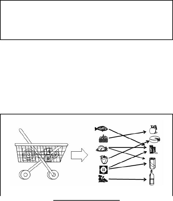
98% of
people who purchased items A
and B
also
purchased item C
Figure-30.1:
Market basket
analysis
249
Lets
consider an example for
better understanding of the
market basket analysis. Figure
30.1
shows a
basket having items A , B
and Y. The right side
portion of the Figure shows
different
items
arranged in two columns and
arrows show the associations
i.e. if item in the left column
is
bought then
the respective item in the
right column is also bought.
How we came to know
this?
This knowledge
was hidden deep in the data,
so querying was not possible
because a store may
contain
thousands of items and
effort to find item associations
trivially is impossible, an NP
complete
problem.
Discovering
Association Rules
�
Given a
set of records, each containing
set of items
� Produce
dependency rules that predict
occurrences of an item based on
others
�
Applications:
� Marketing,
sales promotion and shelf
management
� Inventory
management
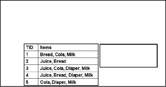
Rules:
{Milk}
�
{Cola}
{Diaper,
Milk} � {Juice}
Table
-30.1: Discovering association
rules
Discovering
Association Rules is another
name given to market basket
analysis. Here rules
are
formed
from the dependencies among
data items which can be
used to predict the
occurrence of
an item based on
others e.g. suppose hardware
shop where whenever a customer
buys color tins it
is more
likely that he /she will buy
painting brushes too. So based on
the occurrence or event of
paint purchase,
we can predict the occurrence of item
paint brush. What is the
benefit of knowing
all
this? We have already
discussed this. Now look at
the Table 30.1, here
two columns TIC
(transaction
ID) and other is the list of
items. This is not the
view of a real database, as a
single
column can
not contain multiple entries
like items column here. This
is an example table just
to
show
rule formation process.
Looking at the table we come
to know that whenever milk
is
purchased,
cola is also purchased. Similarly,
whenever diaper and milk are
purchased juice is also
purchased.
So, the two association
rules are obtained from
the sample data in Table
30.1. Now a
question
arises which of the two
rules strongly implies? This
can not be answered depending on
a
lot of
factors. However, we can
tell what has been discovered
here? What is the
unknown
unknown? The
discovery is that the sale of juice
with diapers and milk is non
trivial. This can
never be
guessed because no obvious
association is found among
the items.
250

CLUSTERING
Task of
segmenting a heterogeneous population
into a number of more homogenous
sub-
groups or
clusters.
Unlike
classification, it does NOT
depend on predefined classes.
It is up to you to
determine what meaning, if any, to
attached to resulting clusters.
It could be the
first step to the market
segmentation effort.
What
else data mining can
do? We can do clustering
with DM. Clustering is the
technique of
reshuffling,
relocating exiting segments in given
data which is mostly
heterogeneous so that
the
new
segments have more homogeneous
data items. This can be
very easily understood by
a
simple
example. Suppose some items
have been segmented on the
basis of color in the given
data.
Suppose
the items are fruits,
then the green segment
may contain all green
fruits like apple,
grapes
etc. thus a heterogeneous mixture of
items. Clustering segregates such
items and brings all
apples in
one segment or cluster although it
may contain apples of
different colors red,
green,
yellow
etc. thus a more homogeneous
cluster than the previous
cluster.
Clustering is a
difficult task, why? In case of
classification we already know
the number of
classes, either
good or bad or yes or no or any number of
classes. We also have the
knowledge of
classes
properties so its easy to
segment data into known
classes. However, in case of
clustering
we don't
know the number of clusters a
priori. Once clusters are
found in the data
business
intelligence, domain
knowledge is needed to analyze the
found clusters. Clustering can be
the
first
step towards market
segmentation i.e. we can use
countermining to know the
possible
clusters in
the data. Once clusters
found and analyzed
classification can be applied thus
gaining
more accuracy
than any standalone
technique. Thus clustering is at higher
level than
classification
not only
because of its complexity but also
because it leads to
classification.
Examples of
Clustering Applications
�
Marketing:
Discovering distinct groups in
customer databases, such as
customers who
make
lot of long-distance calls
and don't have a job.
Who are they? Students.
Marketers
use
this knowledge to develop targeted
marketing programs.
�
Insurance:
Identifying groups of crop insurance
policy holders with a high
average claim
rate.
Farmers crash crops, when it is
"profitable".
�
Land
use: Identification of areas of
similar land use in a GIS
database.
�
Seismic
studies: Identifying probable areas
for oil/gas exploration based on
seismic data.
We discussed
that what clustering is and
how it works. Now to know
the real spirit of it, lets
look
at some of
the real world examples to
show the blessings of
clustering;
1. Knowing
or discovering about your
market segment: Suppose a
telecom company whose
data
when clustered revealed that
there is a group or cluster of people or
customers whose
251
long
distance calls are greater
in number. Is this a discovery that
such a group exi sts?
Nope
not really.
The real discovery is analyzing the
cluster, the real fun part.
Why these people are
in a cluster? Is
important to know. Analysis of the
cluster reveals that all the
people in the
group
are unemployed! How come it
is possible that unemployed
people are making
expensive
far distance calls? The
excitement lead to further
analysis which ultimately
revealed that
the people in the cluster
were mostly students, students
like you living away
from
home in universities , colleges and
hostels. They are making
calls back home. So this
is
a real
example of clustering. Now
the same question what is
the benefit of knowing al
this?
The
answer is customer is like an
asset for any organization. To
know the customer is
crucial
for
any organization/compa ny so as to
satisfy the customer which
is a key of any company's
success in
terms of profit. The company
can rum targeted sale
promotion and marketing
effort to
target customers i.e.
students.
2.
Insurance: Now
lets have look at how
clustering plays a role in
insurance sector.
Insurance
companies
are interested in knowing
the people having higher
insurance claim. You
may
astonish
that clustering has successfully
been used in a developed country to
detect farmer
insurance
abuses. Some of the
malicious farmers used to crash
their crops intentionally to
gain insurance
money which presumably was
higher than the amount of
profit and effort
from
their crops.
The farmer was happy
but the loss was to be
bear by the insurance
company. The
company
successfully used clustering techniques
to identify such farmers,
and thus saving a
lot of
money.
Clustering thus
has a wider scope in real
life applications. Other areas where
clustering is being
used
are for city planning, GIS
(Land use management),
seismic data for mining
(real mining)
and
the list goes on.
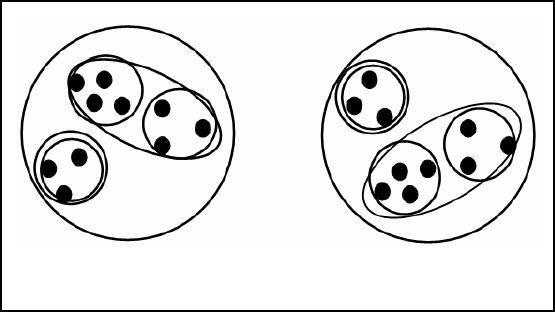
Ambiguity
in Clustering
How
many clusters?
o Two
clusters
o Four
clusters
o Six
clusters
Figure-30.2:
Ambiguity in Clustering
As we mentioned
the spirit of clustering lies in
its analysis. A common ambiguity in
clustering is
regarding the
number of clusters, since the
cluster are not known in
advance. To understand
the
problem,
consider the example in Figure
30.2. The black dots
represent individual data
records or
252
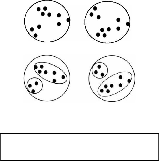
tuples
and they are placed as a
result of a clustering algorithm. Now
can u tell how many
clusters
are
there?
Yes
two clusters, but look at
your screens again and tell
how many clusters
now?
Yes
four clusters now, you are
absolutely right. Now look
again and tell how ma ny
clusters? Yes
6 clusters as
shown in the Figure 30.2.
What all this shows?
This shows that deciding upon
the
number of
clusters is a complex task
depending on factors like
level of detail, application
domain
etc. By
level of detail I mean that either
the black point represents a
single record or an aggregate.
The
thing which is important is to know
how many clusters solve
our problem. Understanding
this
solves the problem.
DESCRIPTION
Describe what is
going on in a complicated database so as
to increas e our
understanding.
A good
description of a behavior will
suggest an explanation as
well.
Another
application of DM is description. To know what is
happening in our databases is
beneficial. How?
The OLAP cubes provide
ample amount of information, which is
otherwise
distributed in
the haystack. We can move
the cube in different angles
to get to the information
of
interest.
However, we might miss the
angle which might have given
use some useful
information.
Description is
used to describe such
things.
253

Comparing
Methods (1)
�
Predictive
accuracy: this refers to
the ability of the model to correctly
predict the class
label of new or
previously unseen
data
�
Speed: this
refers to the computation
costs involved in generating
and using the
method.
�
Robustness: this is
the ability of the method to
make correct predictions/groupings
given
noisy
data or data with missing
values
We discussed
different data mining
techniques. Now the
question, which technique is good
and
which
bad? Or say like which is
the best technique for a
given problem. Thus we need to
specify
evaluation criteria
like data metrics as we did
in the data quality lecture.
The metrics we use
for
comparison of DM
techniques are;
Accuracy:
Accuracy is
the measure of correctness of
your model e.g. in classification we
have
two
data sets, training and
test sets. A classification model is
built based on the data
properties
and
relationships in training data.
Once built the model is
tested for accuracy in terms
of %
correct
results as the classification of
the test data is already
known. So we specify the
correctness
or confidence
level of the technique in
terms % accuracy.
Speed:
In
previous lectures we discussed
the term "Need for Speed".
Yes speed is a crucial
aspect of Dm
techniques. Speed refers to
the time complexity. If a technique has O
(n) and
another
has O (n log n) time complexities
then which is better? Yes O
(n) is better. This is
the
computational time but
user or business decision
maker is interested in the
absolute clock time.
He has nothing
to do with complexities. What he is
interested in is, knowing
how fast he gets
the
answers. So
just comparing on the basis of
complexities is not sufficient. We must
look at the
overall
process and interdependencies
among tasks which ultimately
result in the answer
or
information
generation.
Robustness:
It is
the ability of the technique
to work accurately even in
conditions of noisy or
dirty
data. Missing data is a reality
and presence of noise also
true. So a technique is better if
it
can
run smoothly even in stress
conditions i.e. with noisy
and missing data.
Scalability:
As we
mentioned in our initial
lectures that the main
motivation for data
warehousing is to
deal huge amounts of data.
So scaling is very important, which is
the ability of
the
method to work efficiently even when
the data size is
huge.
Interpretability:
It refers to
the level of understanding
and insight that is provided by
the
method. As we
discussed in clustering one of the
complex and difficult tasks is
the cluster
analysis.
The techniques can be
compared on the basis of
their interpretational ability e.g.
there
might be
some methods which give
additional functionalities to provide
meaning to the
discovered
information like color
coding, plots and curve
fittings etc.
254
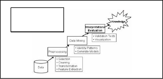
Where
does Data Mining fits
in?
Data
Mining is one step
of
Knowledge
Discovery in
Databases
(KDD)
Figure-30.3:
Where does Data Mining fits
in?
Now
lets look at the overall
knowledge discovery KD process. Figure
30.3 shows different
KDD
steps.
Data is crucial and the most
important component of KDD, knowledge discovery
is
possible
only if data is available. The
data is not used in its
crude form for knowledge
discovery.
Before
applying analysis techniques
like data mining, data is
preprocessed using activities as
discussed in
ETL. You ca n see an
additional process at the
preprocessing step i.e.
feature
extraction.
This is to extract those
data items which are
needed or which or of interest
form the
huge
data set. Suppose we have an
O (n2) method for
data processing. Scalability can be
issue for
large data
sets because of quadratic
nature. The problem can be solved if we
perform aggregation,
reducing number
of records and keeping the
data properties. So now the
method can work
with
less
data size. Next comes the
data mining phase, we have
thoroughly discussed the
techniques
for
discovering patterns (clustering) and
generating models (classification). The
next step is the
analysis of
discovered patterns using domain
knowledge. This is a complex task
and requires an
ample
amount of business or domain knowledge.
The interpreted knowledge finally
comes out as
the
information that was unknown
before hidden in the data
sea which has now
become
information
having some value to the
user.
255
Table of Contents:
- Need of Data Warehousing
- Why a DWH, Warehousing
- The Basic Concept of Data Warehousing
- Classical SDLC and DWH SDLC, CLDS, Online Transaction Processing
- Types of Data Warehouses: Financial, Telecommunication, Insurance, Human Resource
- Normalization: Anomalies, 1NF, 2NF, INSERT, UPDATE, DELETE
- De-Normalization: Balance between Normalization and De-Normalization
- DeNormalization Techniques: Splitting Tables, Horizontal splitting, Vertical Splitting, Pre-Joining Tables, Adding Redundant Columns, Derived Attributes
- Issues of De-Normalization: Storage, Performance, Maintenance, Ease-of-use
- Online Analytical Processing OLAP: DWH and OLAP, OLTP
- OLAP Implementations: MOLAP, ROLAP, HOLAP, DOLAP
- ROLAP: Relational Database, ROLAP cube, Issues
- Dimensional Modeling DM: ER modeling, The Paradox, ER vs. DM,
- Process of Dimensional Modeling: Four Step: Choose Business Process, Grain, Facts, Dimensions
- Issues of Dimensional Modeling: Additive vs Non-Additive facts, Classification of Aggregation Functions
- Extract Transform Load ETL: ETL Cycle, Processing, Data Extraction, Data Transformation
- Issues of ETL: Diversity in source systems and platforms
- Issues of ETL: legacy data, Web scrapping, data quality, ETL vs ELT
- ETL Detail: Data Cleansing: data scrubbing, Dirty Data, Lexical Errors, Irregularities, Integrity Constraint Violation, Duplication
- Data Duplication Elimination and BSN Method: Record linkage, Merge, purge, Entity reconciliation, List washing and data cleansing
- Introduction to Data Quality Management: Intrinsic, Realistic, Orr’s Laws of Data Quality, TQM
- DQM: Quantifying Data Quality: Free-of-error, Completeness, Consistency, Ratios
- Total DQM: TDQM in a DWH, Data Quality Management Process
- Need for Speed: Parallelism: Scalability, Terminology, Parallelization OLTP Vs DSS
- Need for Speed: Hardware Techniques: Data Parallelism Concept
- Conventional Indexing Techniques: Concept, Goals, Dense Index, Sparse Index
- Special Indexing Techniques: Inverted, Bit map, Cluster, Join indexes
- Join Techniques: Nested loop, Sort Merge, Hash based join
- Data mining (DM): Knowledge Discovery in Databases KDD
- Data Mining: CLASSIFICATION, ESTIMATION, PREDICTION, CLUSTERING,
- Data Structures, types of Data Mining, Min-Max Distance, One-way, K-Means Clustering
- DWH Lifecycle: Data-Driven, Goal-Driven, User-Driven Methodologies
- DWH Implementation: Goal Driven Approach
- DWH Implementation: Goal Driven Approach
- DWH Life Cycle: Pitfalls, Mistakes, Tips
- Course Project
- Contents of Project Reports
- Case Study: Agri-Data Warehouse
- Web Warehousing: Drawbacks of traditional web sear ches, web search, Web traffic record: Log files
- Web Warehousing: Issues, Time-contiguous Log Entries, Transient Cookies, SSL, session ID Ping-pong, Persistent Cookies
- Data Transfer Service (DTS)
- Lab Data Set: Multi -Campus University
- Extracting Data Using Wizard
- Data Profiling