Transportation Problems:TRANSPORTATION MODEL, Distribution centers

<< Linear Programming:Multiple or Alternative optimal Solutions

Transportation Problems:FINDING AN INITIAL BASIC FEASIBLE SOLUTION >>

Operations Research (MTH601)

164

Segment V: Transportation Problems

Lectures 31- 35

164

Operations Research (MTH601)

165

INTRODUCTION

Many practical problems in operations research can be broadly formulated as linear programming

problems, for which the simplex this is a general method and cannot be used for specific types of problems like,

(i)

transportation models,

(ii)

transshipment models and

(iii)

the assignment models.

The above models are also basically allocation models. We can adopt the simplex technique to solve

them, but easier algorithms have been developed for solution of such problems. The following sections deal

with the transportation problems and their streamlined procedures for solution.

TRANSPORTATION MODEL

In a transportation problem, we have certain origins, which may represent factories where we produce

items and supply a required quantity of the products to a certain number of destinations. This must be done in

such a way as to maximize the profit or minimize the cost. Thus we have the places of production as origins and

the places of supply as destinations. Sometimes the origins and destinations are also termed as sources and

sinks.

To illustrate a typical transportation model, suppose m factories supply certain items to n warehouses.

Let factory i (i = 1, 2, ..., m) produce ai units and the warehouse j (j = 1, 2, ..., n) requires bj units. Suppose the

cost of transportation from factory i to warehouse j is cij. Let us define the decision variables xij being the

amount transported from the factory i to the warehouse j. Our objective is to find the transportation pattern that

will minimize the total transportation cost.

The model of a transportation problem can be represented in a concise tabular form with all the

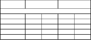
relevant parameters mentioned above. See table 1

Table 1

Origins

Destinations

Available

(Factories)

(Warehouses)

........

c11

c12

c1n

c21

c22

c2n

...

...

cm1

cm2

cmn

Required

The pattern of distribution of items in the form of transportation matrix is separately given below in table 2.

165

Operations Research (MTH601)

166

Table 2

Origins

Destinations

Available

2 ........

x11

x12

x1n

x21

x22

x2n

...

xm1

xm2

xmn

Required

TRANSPORTATION PROBLEM AS AN L.P MODEL

The transportation problem can be represented mathematically as a linear programming model. The

objective function in this problem is to minimize the total transportation cost given by

Z = c11 x11 + c12x12 + ... + cmn xmn

Subject to the restrictions:

row restrictions

x11 + x12 +

+ x1n = a1

x21 + x22 +

+ x2n = a2

xm1 + xm2 +

+ xm1 = am

Column restrictions

x11 + x21 +

+ xm1 = b1

x12 + x22 +

+ xm2 = b2

x1n + x2n +

+ xmn = bn

and

x11 , x12 , ... , xmn ≥ 0

It should be noted that the model has feasible solutions only if

a +a +

+ am = b1 + b2 + + bn

∑ a1

= ∑ bj

i=1

j =1

The above is a mathematical formulation of a transportation problem and we can adopt the linear

programming technique with equality constraints. Here the algebraic procedure of the simplex method may not

166

Operations Research (MTH601)

167

be the best method to solve the problem and hence more efficient and simpler streamlined procedures have

been developed to solve transportation problems.

Example 1 (Formulation of a transportation problem)

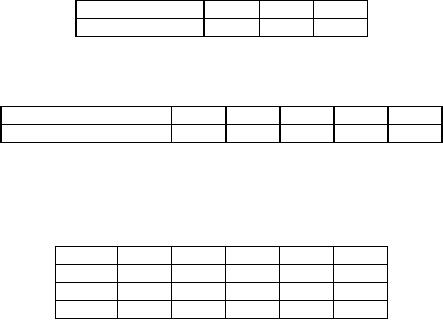
A company has plants located at three places where the production pattern is described in the following table.

Plant location

Production (units)

The potential demand at five places has been estimated by the marketing department and is presented below.

Distribution centre

Potential demand (units)

The cost of transportation from a plant to the distribution centre has been displayed in the table

Table 3

Distribution centers

Plant

Represent the above data in a table to represent a transportation problem.

Solution:

In this example the total supply and the total demand do not match as supply is less than demand.

Hence a dummy row (dummy plant) is introduced at a unit transportation cost of 0. The following is the tabular

representation of the transportation problem.

Note: If the total demand (requirements) is less than the total supply (availability), a dummy column (dummy

destination) is introduced with a unit transportation cost of 0.

167

Table of Contents: