 |
Transportation Problems:DEGENERACY, Destination |
| << Transportation Problems:MOVING TOWARDS OPTIMALITY |
| Transportation Problems:REVIEW QUESTIONS >> |
Operations
Research (MTH601)
195
a)
Develop an optimum transportation
schedule and give the
minimum transportation
cost.
b) Is it
possible to have more than
one optimum schedule? If so,
give at least one more
optimum
schedule.
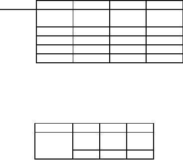
13.
Peru
enterprise has three
factories at location A, B and C, which
supplies three warehouses,
located at
D,
E and F. Monthly factory capacities
are 10, 18 and 15 units
respectively. Monthly
warehouse
requirements
are 75, 20 and 50 units
respectively.
Warehouse
Factory
D
E
F
A
5
1
7
B
6
4
6
C
3
2
5
The
penalty costs for not
satisfying demand at the warehouses
D,
E and
F
are
Rs. 5, Rs. 3, and Rs.
2
per
unit respectively. Determine
the optimal distribution for
Peru using any of the
known algorithms.
14.
A
fleet operator has in his
three depots P, Q and R 1
bus and 8 buses and 7
buses respectively. He
has
to
allocate them to those bus
stands X, Y and Z, which
require 2, 5 and 9 buses
respectively. The
following
table gives the distances in
kilometers from each depot to
each bus stand. Find
the optimum
allocation.
X
Y
Z
P
6
4
12
Q
10
6
5
R
15
16
8
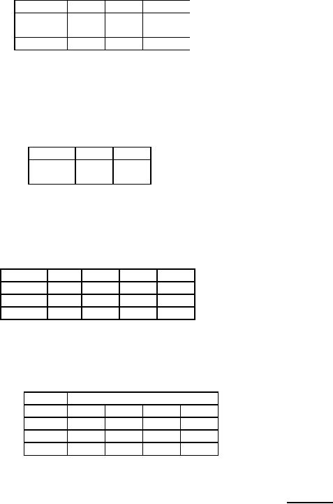
15.
A
firm has 4 factories, which
produce 8, 7, 9 and 4 units
respectively of a product. The
firm owns three
stores,
which sells 8 units
respectively. The unit
transportation cost is given
below in the table.
Store
Factory
A
B
C
P
10
9
8
Q
10
7
10
R
11
9
7
S
12
14
10
Find
the transportation schedule,
which minimizes the distribution
cost.
DEGENERACY
In
the examples discussed so
far, the solution procedure
yielded exactly (m + n - 1) strictly
positive
allocations,
in independent positions indicating
non-degenerate basic feasible
solution. When either of
the
conditions
for conducting optimality is
absent it results in a degenerate
solutions. The circumstances in
many
cases
may not yield result,
which satisfy conditions for
optimality tests. We may
have less number of
cells
alloted
even in the initial basic
feasible solution, found,
either by North West Corner
rule or other methods
described
previously. It may be sometimes non-degenerate in
the initial basic feasible
solution but at any
intermediate
iteration (while we conduct
the optimality test) it may
lead to a case of a degenerate
feasible
solution.
This particularly occurs when a row
and a column simultaneously vanish,
while making allocations
initially
by any of the methods. Th
situation of degeneracy can be
resolved as explained in the
next paragraph.
195
Operations
Research (MTH601)
196
A
feasible solution with independence,
but with fewer than the
required number of
individual
allocations
is changed to become permissible in
the following way. We have
to choose the required
number of
cells,
such that this number plus
the existing allocation come to exactly
(m
+ n - 1)
cells should be in
independent
positions. Then, an infinitesimal
but positive allocation, say an
amount equal to is allotted to
each
of
the chosen unoccupied cells.
This fictitious allotment does not
change the physical nature
of the original set
of
allocations, but will be helpful to
carry out the iterations.
This small fictitious quantity plays an
auxiliary role
and
it is removed when the
optimum is reached.
Sometimes
a feasible solution may degenerate to
m
+ n - 3 or
even fewer independent allocations.
In
such
cases, if the transportation
method is to be adopted in finding a
solution to the problem, we will
have to
introduce
two or more infinitesimal
variables (∈).
The ∈'s
are also placed in various
independent positions
and
can
be distinguished from each
other by subscripts.
Example:
Solve the following
transportation problem to minimize
the total cost of
transportation.
Destination
Origin
1
2
3
4
Supply
1
14
56
48
27
70
2
82
35
21
81
47
3
99
31
71
63
93
Demand
70
35
45
60
210
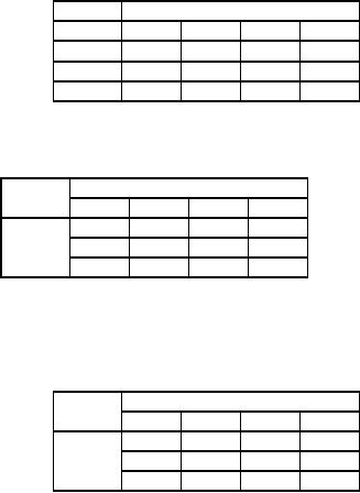
Solution:
First
obtain an indicial basic
feasible solution with Vogel's
Approximation Method from the
table 62
Table
62
Destination
Origin
1
2
3
4
Supply
Penalty
70
14
1
56
48
27
70
(13)
2
82
35
21
81
47
(14)
3
99
31
71
63
93
(32)
Demand
70
35
45
60
210
Penalty
(68)
(4)
(36)
(36)
Supply
70 to 1 from 1. Hence row 1
and column 1 are both eliminated.
The reduced matrix is shown
in table 63
Table
63
Destination
Origin
2
3
4
Supply
Penalty
45
21
2
35
81
47
(14)
3
31
71
63
93
(32)
Demand
35
45
60
140
Penalty
(4)
(50)
(18)
Supply
45 to 3 from 2 and hence column 3 is
eliminated, resulting in table 64
196
Operations
Research (MTH601)
197
Table
64
Destination
Origin
2
4
Supply
2
2
35
81
2
(46)
3
63
93
(32)
Demand
35
60
95
Penalty
(4)
(18)
Supply
35 items from origin 2 to
destination 2 and row 2 is
deleted.
Table
65
Destination
Origin
2
4
Supply
33
60
31
63
3
93
Demand
33
60
93
Summarising
the above results we have
the initial feasible allocation as
exhibited in table 66
Table
66
Destination
Origin
1
2
3
4
Supply
1
70
70
2
2
45
47
3
33
60
93
Demand
Cost:
70 x 14 + 2 x 35 + 45 x 21 + 33 x 31 + 60 x 63 = Rs.
6798/-
Table
67
Destination
Origin
1
2
3
4
1
14
56
48
27
2
82
35
21
81
3
99
31
31
63
Cost
matrix
To
conduct the optimality test
for the above solution there
must be 6 ( = 3 + 4 - 1) cells to
which
allocation
must have been made.
But we have made allotment to 5
cells only. Hence this is a
degenerate basic
feasible
solution.
To
resolve the case of
degeneracy, we introduce a very
small quantity ∈
in a
vacant and
independent
cell.
In the above problem we
allot ∈
to
cell (1, 4), which is
independent. The optimality
test can now be
conducted
as shown in the following
tables 68 to 72.
197
Operations
Research (MTH601)
198
Table
68
Destination
Origin
1
2
3
4
∈
1
70
2
2
45
3
33
60
Allotment
matrix
Table
69
Destination
Origin
ui
1
2
3
4
1
14
-
-
27
0
u1
2
-
35
21
-
40
u2
3
36
-
31
63
u3
vj
v1
v2
v3
v4
14
-5
-19
27
Cost
of alloted cells and
(ui + vj)
Table
70
Destination
Origin
1
2
3
4
1
56
48
2
82
81
3
99
71
Cost
of unalloted cells
198
Table of Contents:
- Introduction:OR APPROACH TO PROBLEM SOLVING, Observation
- Introduction:Model Solution, Implementation of Results
- Introduction:USES OF OPERATIONS RESEARCH, Marketing, Personnel
- PERT / CPM:CONCEPT OF NETWORK, RULES FOR CONSTRUCTION OF NETWORK
- PERT / CPM:DUMMY ACTIVITIES, TO FIND THE CRITICAL PATH
- PERT / CPM:ALGORITHM FOR CRITICAL PATH, Free Slack
- PERT / CPM:Expected length of a critical path, Expected time and Critical path
- PERT / CPM:Expected time and Critical path
- PERT / CPM:RESOURCE SCHEDULING IN NETWORK
- PERT / CPM:Exercises
- Inventory Control:INVENTORY COSTS, INVENTORY MODELS (E.O.Q. MODELS)
- Inventory Control:Purchasing model with shortages
- Inventory Control:Manufacturing model with no shortages
- Inventory Control:Manufacturing model with shortages
- Inventory Control:ORDER QUANTITY WITH PRICE-BREAK
- Inventory Control:SOME DEFINITIONS, Computation of Safety Stock
- Linear Programming:Formulation of the Linear Programming Problem
- Linear Programming:Formulation of the Linear Programming Problem, Decision Variables
- Linear Programming:Model Constraints, Ingredients Mixing
- Linear Programming:VITAMIN CONTRIBUTION, Decision Variables
- Linear Programming:LINEAR PROGRAMMING PROBLEM
- Linear Programming:LIMITATIONS OF LINEAR PROGRAMMING
- Linear Programming:SOLUTION TO LINEAR PROGRAMMING PROBLEMS
- Linear Programming:SIMPLEX METHOD, Simplex Procedure
- Linear Programming:PRESENTATION IN TABULAR FORM - (SIMPLEX TABLE)
- Linear Programming:ARTIFICIAL VARIABLE TECHNIQUE
- Linear Programming:The Two Phase Method, First Iteration
- Linear Programming:VARIANTS OF THE SIMPLEX METHOD
- Linear Programming:Tie for the Leaving Basic Variable (Degeneracy)
- Linear Programming:Multiple or Alternative optimal Solutions
- Transportation Problems:TRANSPORTATION MODEL, Distribution centers
- Transportation Problems:FINDING AN INITIAL BASIC FEASIBLE SOLUTION
- Transportation Problems:MOVING TOWARDS OPTIMALITY
- Transportation Problems:DEGENERACY, Destination
- Transportation Problems:REVIEW QUESTIONS
- Assignment Problems:MATHEMATICAL FORMULATION OF THE PROBLEM
- Assignment Problems:SOLUTION OF AN ASSIGNMENT PROBLEM
- Queuing Theory:DEFINITION OF TERMS IN QUEUEING MODEL
- Queuing Theory:SINGLE-CHANNEL INFINITE-POPULATION MODEL
- Replacement Models:REPLACEMENT OF ITEMS WITH GRADUAL DETERIORATION
- Replacement Models:ITEMS DETERIORATING WITH TIME VALUE OF MONEY
- Dynamic Programming:FEATURES CHARECTERIZING DYNAMIC PROGRAMMING PROBLEMS
- Dynamic Programming:Analysis of the Result, One Stage Problem
- Miscellaneous:SEQUENCING, PROCESSING n JOBS THROUGH TWO MACHINES
- Miscellaneous:METHODS OF INTEGER PROGRAMMING SOLUTION