THE PARTS OF THE TABLE:Reading a percentage Table

<< DATA PRESENTATION:Bivariate Tables, Constructing Percentage Tables

EXPERIMENTAL RESEARCH:The Language of Experiments >>

Research Methods STA630

Lesson 32

THE PARTS OF THE TABLE

Give each table a number.

Give each table a title, which names variables and provides background information

Label the row and columns variables and give name to each of the variable categories.

Include the totals of the columns and rows. These are called marginals.They equal the

univariate frequency distribution for the variable.

5. Each number or place that corresponds to the intersection of a category for each variable is a

cell of a table.

6. The numbers with the labeled variable categories and the totals are called the body of the table.

7. If there is missing information, report the number of missing cases near the table to account for

all original cases.

Researchers convert raw count tables into percentages to see bi-variate relationship. There are three

ways to percentage a table: by row, by column, and for the total. The first two are often used and show

relationship.

Is it best to percentage by row or column? Either could be appropriate. A researcher's hypothesis may

imply looking at row percentages or the column percentages. Here, the hypothesis is that age affects

attitude, so column percentages are most helpful. Whenever one factor in a cross-tabulation can be

considered the cause of the other, percentage will be most illuminating if they are computed in the

direction of the causal factor.

Reading a percentage Table: Once we understand how table is made, reading it and figuring out what

it says are much easier. To read a table, first look at the title, the variable labels, and any background

information. Next, look at the direction in which percentages have been computed in rows or

columns.

Researchers read percentaged tables to make comparisons. Comparisons are made in the opposite

direction from that in which percentages are computed. A rule of thumb is to compare across rows if the

table is percentaged down (i.e. by column) and to compare up and down in columns if the table is

percentaged across (i.e. by row).

It takes practice to see a relationship in a perentaged table. If there is no relationship in a table, the cell

percentages look approximately equal across rows or columns. A linear relationship looks like larger

percentages in the diagonal cells. If there is curvilinear relationship, the largest percentages form a

pattern across cells. For example, the largest cells might be the upper right, the bottom middle, and the

upper left. It is easiest to see a relationship in a moderate-sized table (9 to 16 cells) where most cells

have some cases (at least five cases are recommended) and the relationship is strong and precise.

Linear relationship

· Table 4: Age by attitude towards women

empowerment

Age (in years)

Level of

under 40

40 60

61 +

Total

attitude

Hi Favorable

600

300

200

1100

Med. Favorable 300

500

250

1050

Lo Favorable

100

200

500

850

Total

1000

100

1000 100

1000

100

3000

100

Larger percentages in the diagonal cells

107

Research Methods STA630

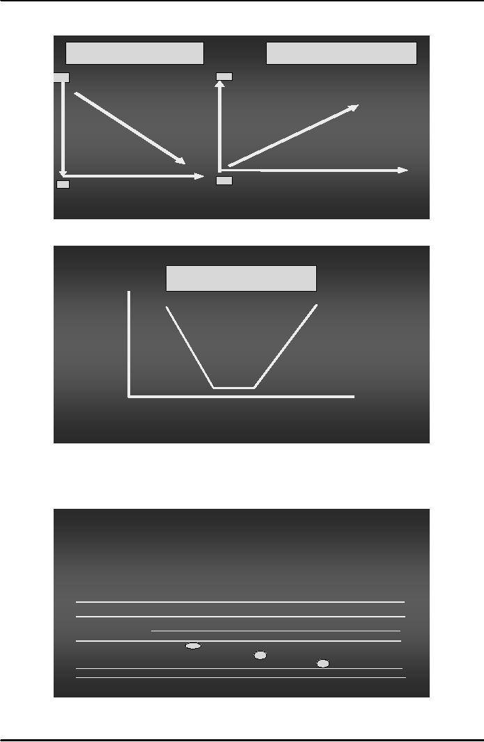
Linear

Negative relationship

Positive relationship

Curvilinear

A simple way to see strong relationships is to circle the largest percentage in each row (in row

percentaged tables) or columns (for column-percentaged tables) and see if a line appears.

A simple way to see strong relationship is to

circle the largest percentage in applicable

row or column and see if a line appears

· Table 4: Age by attitude towards women

empowerment

Age (in years)

Level of

under 40

40 60

61 +

Total

attitude

Hi Favorable

600

300

200

1100

Med. Favorable 300

500

250

1050

Lo Favorable

100

200

500

850

Total

1000

100

1000 100

1000

100

3000

100

108

Research Methods STA630

The circle-the-largest-cell rule works with one important caveat. The categories in the percentages

table must be ordinal or interval. The lowest variable categories begin at the bottom left. If the

categories in a table are not ordered the same way, the rule does not work.

Statistical Control

Showing an association or relationship between two variables is not sufficient to say that an independent

variable causes a dependent variable. In addition to temporal order and association, a researcher must

eliminate alternative explanations explanations that can make the hypothetical relationship spurious.

Experimental researchers do this by choosing a research design that physically controls potential

alternative explanations for results (i.e. that threaten internal validity).

In non-experimental research, a researcher controls for alternative explanations with statistics. He or

she measures possible alternative explanations with control variables, and then examines the control

variables with multivariate tables and statistics that help him or her to decide whether a bivariate

relationship is spurious. They also show the relative size of the effect of multiple independent variables

on dependent variable.

A researcher controls for alternative explanation in multivariate (more than two variables) analysis by

introducing a third (sometimes fourth, or fifth) variable. For example, a bivariate table shows that

young people show more favorable attitude towards women empowerment. But the relationship

between age and attitude towards women empowerment may be spurious because men and women may

have different attitudes. To test whether the relationship is actually due to gender, a researcher must

control for gender; in other words, effects of gender are statistically removed. Once this is done, a

researcher can see whether the bivariate relationship between age and attitude towards women

empowerment remains.

A researcher controls for a third variable by seeing whether the bivariate relationship persists within

categories of the control variable. For example controls for gender, and the relationship between age

and attitude persists. This means that both male and females show negative association between age

and attitude toward women empowerment. In other words, the control variable has no effect. When

this is so, the bivariate relationship is not spurious.

If the bivariate relationship weakens or disappears after the control variable is considered, it means that

the age is not real factor that makes the difference in attitude towards women empowerment, rather it is

the gender of the respondents.

Statistical control is a key idea in advanced statistical techniques. A measure of association like the

correlation co-efficient only suggests a relationship. Until a researcher considers control variables, the

bivariate relationship could be spurious. Researchers are cautious in interpreting bivariate relationships

until they have considered control variables.

After they introduce control variables, researchers talk about the net effect of an independent variable

the effect of independent variable "net of," or in spite of, the control variable. There are two ways to

introduce control variables: trivariate percentaged tables and multiple regression analysis.

Constructing Trivariate Tables

In order to meet all the conditions needed for causality, researchers want to "control for" or see whether

an alternative explanation explains away a causal relationship. If an alternative explanation explains a

relationship, then bivariate relationship is spurious. Alternative explanations are operationalize as a

third variable, which are called control variables because they control for alternative explanation.

109

Research Methods STA630

One way to take such third variables into consideration and see whether they influence the bivariate

relationship is to statistically introduce control variables using trivariate or three variable tables.

Trivariate tables differ slightly from bivariate tables; they consist of multiple bivariate tables.

A trivariate table has a bivariate table of the independent and dependent variable for each category of

the control variable. These new tables are called partials. The number of partials depends on the

number of categories in control variable. Partial tables look like bivariate tables, but they use a subset

of the cases. Only cases with a specific value on the control variable are in the partial. Thus it is

possible to break apart a bivariate table to form partials, or combine the partials to restore the initial

bivariate table.

Trivariate tables have three limitations. First, they are difficult to interpret if a control variable has more

that four categories. Second, control variables can be at any level of measurement, but interval or ratio

control variables must be grouped (i.e. converted to an ordinal level), and how cases are grouped can

affect the interpretation of effects. Finally, the total number of cases is a limiting factor because the

cases are divided among cells in partials. The number of cells in the partials equals the number of cells

in the bivariate relationship multiplied by the number of categories in the control variables. For example

if the control variable has three categories, and a bivariate table has 12 cells, the partials have 3 X 12 =

36 cells. An average of five cases per cell is recommended, so the researcher will need 5 X 36 = 180

cases at minimum.

Like a bivariate table construction, a trivariate table begins with a compound frequency distribution

(CFD), but it is a three-way instead of two-way CFD. An example of a trivariate table with "gender" as

control variable for the bivariate table is shown here:

Partial table for males

Age (in years)

Level of

Under 40

40--60

61+

Total

Attitude

High

300

200

6 530

Medium

140

270

120

24 530

Low

130

350

70 540

Total

500

100

600

100

500 100 1600

100

Partial table for females

Age (in years)

Level of

.Under 40

40--60

61+

Total

Attitude

High

350

200

570

Medium

150

220

520

Low

260

310

Total

500

100

400

100

500

100

1400

100

The replication pattern is the easiest to understand. It is when the partials replicate or reproduce the

same relationship that existed in the bivariate table before considering the control variable. It means

that the control variable has no effect.

110

Research Methods STA630

The specification pattern is the next easiest pattern. It occurs when one partial replicate the initial

bivariate relationship but other partials do not. For example, we find a strong (negative) bivariate

relationship between age of the respondents and attitude towards women empowerment. We control for

gender and discover the relationship holds only for males (i.e. the strong negative relationship was in the

partial for males, but not for females). This is specification because a researcher can specify the

category of the control variable in which the initial relationship persists.

The interpretation pattern describes the situation in which the control variable intervenes between the

original independent variable and the dependent variables.

The suppressor variable pattern occurs when the bivariate tables suggest independence but relationship

appears in one or both of the partials. For example, the age of the respondents and their attitudes

towards women empowerment are independent in a bivariate table. Once the control variable "gender"

is introduced, the relationship between the two variables appears in the partial tables. The control

variable is suppressor variable because it suppressed the true relationship; the true relationship appears

in partials.

Multiple Regression Analysis

Multiple regression controls for many alternative explanations of variables simultaneously (it is rarely

possible to use more than one control variable using percentaged tables). Multiple regression is a

technique whose calculation you may have learnt in the course on statistics.

Note

In the preceding discussion you have been exposed to the descriptive analysis of the data. Certainly

there are statistical tests which can be applied to test the hypothesis, which you may have learnt in your

course on statistics.

111

Table of Contents: