 |
Production with Two Variable Inputs:Returns to Scale |
| << The Technology of Production:Production Function for Food |
| Measuring Cost: Which Costs Matter?:Cost in the Short Run >> |
Microeconomics
ECO402
VU
Lesson
17
Production
with Two Variable
Inputs
There is a
relationship between production
and productivity.
Long-run
production K& L are
variable.
Isoquants
analyze and compare the
different combinations of K & L and
output
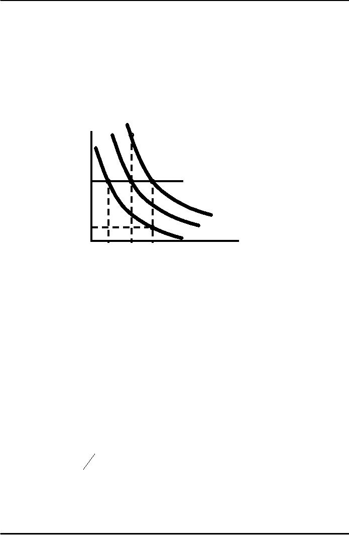
The
Shape of Isoquants
Capital
per
year
E
5
In
the long run
both
4
labor
and capital are
variable
and both
experience
diminishing
3
returns.
A
B
C
2
Q3 =
90
D
Q2 =
75
1
Q1 =
55
1
2
3
4
5
Labor
per year
Diminishing
Marginal Rate of
Substitution
Reading the
Isoquant Model
1)
Assume capital is 3 and
labor increases from 0 to 1 to 2 to
3.
Notice output
increases at a decreasing rate
(55, 20, 15) illustrating
diminishing
returns
from labor in the short-run
and long-run.
2)
Assume labor is 3 and
capital increases from 0 to 1 to 2 to
3.
Output also
increases at a decreasing rate
(55, 20, 15) due to
diminishing returns
from
capital.
Substituting
Among Inputs
Managers want
to determine what combination if
inputs to use.
They must
deal with the trade-off
between inputs.
The slope of
each isoquant gives the
trade-off between two inputs
while keeping output
constant.
The marginal
rate of technical substitution
equals:
MRTS
=
-
Changein
capital/Change in labor
input
MRTS
= -
ΔK
(for
a fixed level of Q)
ΔL
85
Microeconomics
ECO402
VU
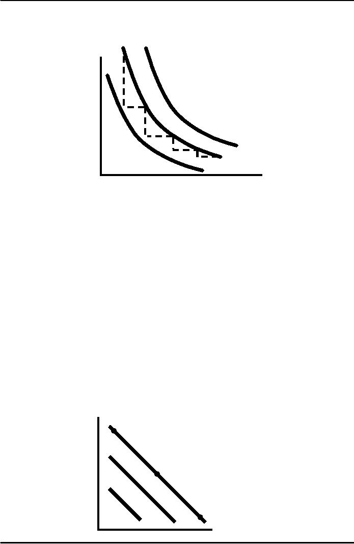
Marginal
Rate of Technical
Substitution
Capital
5
per
year
Isoquants
are downward
sloping
and convex
2
like
indifference
4
curves.
1
3
1
1
2
Q3 =90
2/
1
1/
Q2 =75
1
1
Q1 =55
5
Labor per
month
3
4
2
1
Observations:
1.
Increasing labor in one unit
increments from 1 to 5 results in a
decreasing MRTS from
1
to 1/2.
2.
Diminishing MRTS occurs
because of diminishing returns
and implies isoquants
are
convex.
MRTS
and Marginal
Productivity
·
The change in
output from a change in
labor equals:
(MP
L )( Δ
L)
·
The
change in output from a
change in capital
equals:
)(
Δ
K)
(MP
K
·
If output is
constant and labor is
increased, then:
(MP
L )( Δ
L)
+
(MP
K )( Δ
K)
=
0
(MP
L )(MP K
) =
-
( Δ
K/
Δ
L)
=
MRTS
Isoquants
When Inputs are perfectly
substitutable
A
B
C
Q1
Q2
Q3
Labor
per month
86
Microeconomics
ECO402
VU
Perfect
Substitute
Observations
when inputs are perfectly
substitutable:
1)
The MRTS is constant at all
points on the
isoquant.
2)
For a given output, any
combination of inputs can be
chosen (A, B, or C) to
generate
the same level of output
(e.g. toll booths &
musical instruments).
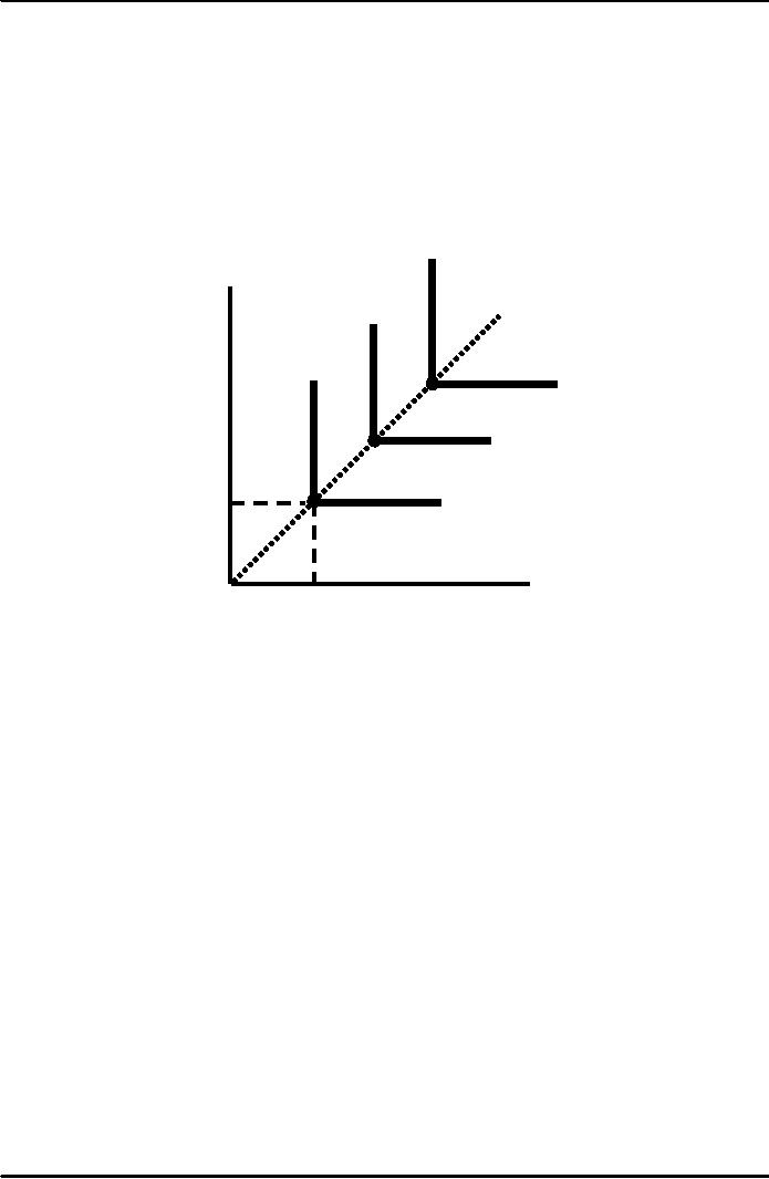
Fixed-Proportions
Production Function
Capital
per
month
Q3
C
Q2
B
Q1
K1
A
Labor
per
month
L1
Fixed-Proportions
Production Function
Observations
when inputs must be in a
fixed-proportion:
1)
No substitution is possible. Each
output requires a specific
amount of each input
(e.g.
labor and
jackhammers).
2)To
increase output requires
more labor and capital
(i.e. moving from A to B to
C
which
is technically efficient).
A
Production Function for
Wheat
Farmers
must choose between a
capital intensive or labor
intensive technique of
production.
87
Microeconomics
ECO402
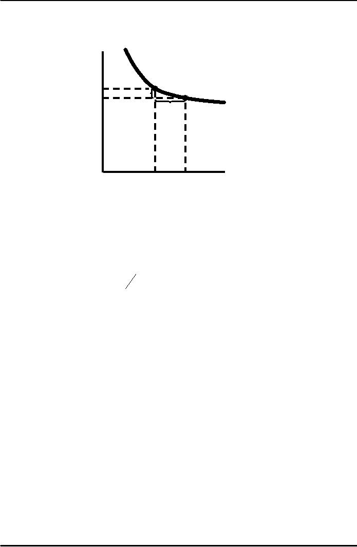
VU
Isoquant
Describing the Production of
Wheat
Capital
(Machine
Point
A is
more
hour
per
capital-intensive,
and
120
year)
B
is
more labor-intensive.
A
100
B
ĆK =
-10
90
ĆL =
260
80
Output
= 13,800 bushels
per
year
40
Labor
250
500
760
1000
(hours
per year)
Observations:
1)
Operating at A:
·
L
= 500 hours and K = 100
machine hours.
2)
Operating at B
·
Increase L to
760 and decrease K to 90 the
MRTS < 1:
MRTS
=
-ΔK
=
-(10 /
260) =
0.04
ΔL
3)
MRTS < 1, therefore the
cost of labor must be less
than capital in order for
the
farmer
substitute labor for
capital.
4)
If labor is expensive, the
farmer would use more
capital (e.g. U.S.).
5)
If labor is inexpensive, the
farmer would use more
labor (e.g. India).
88
Microeconomics
ECO402
VU
Returns
to Scale
Measuring
the relationship between the
scale (size) of a firm and
output
1.
Increasing returns to scale:
output
more than doubles when
all inputs are
doubled
Larger output
associated with lower cost
(autos)
One firm is
more efficient than many
(utilities)
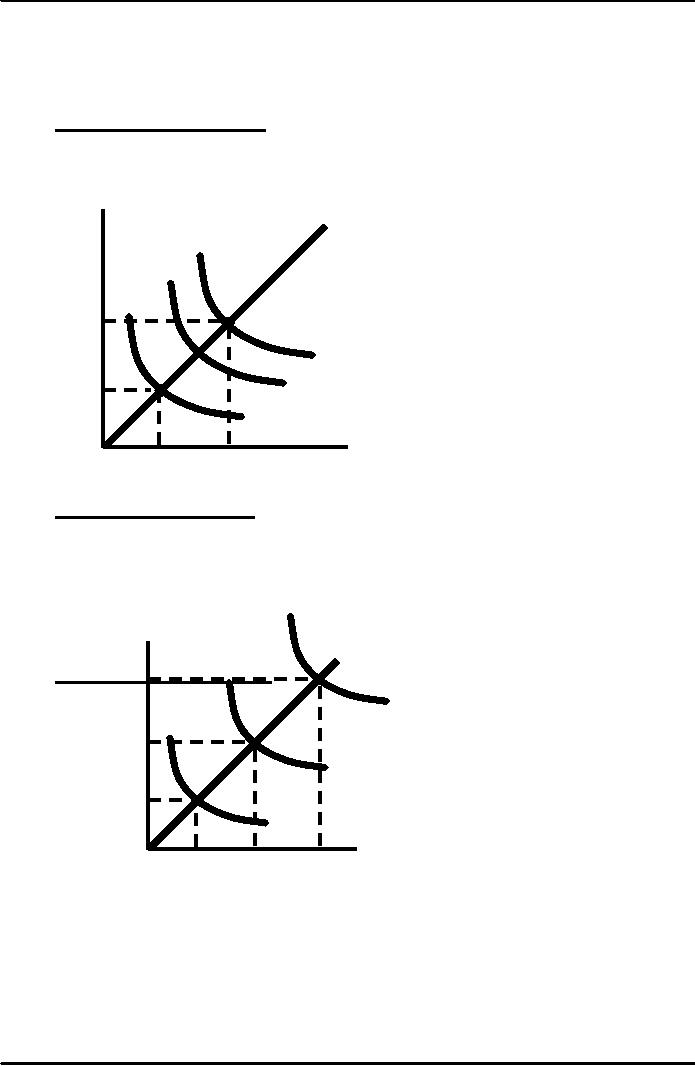
The isoquants
get closer together
Increasing
Returns:
Capital
A
The
isoquants move closer
(machine
together
hours)
4
30
20
2
10
Labor
(hours)
0
5
10
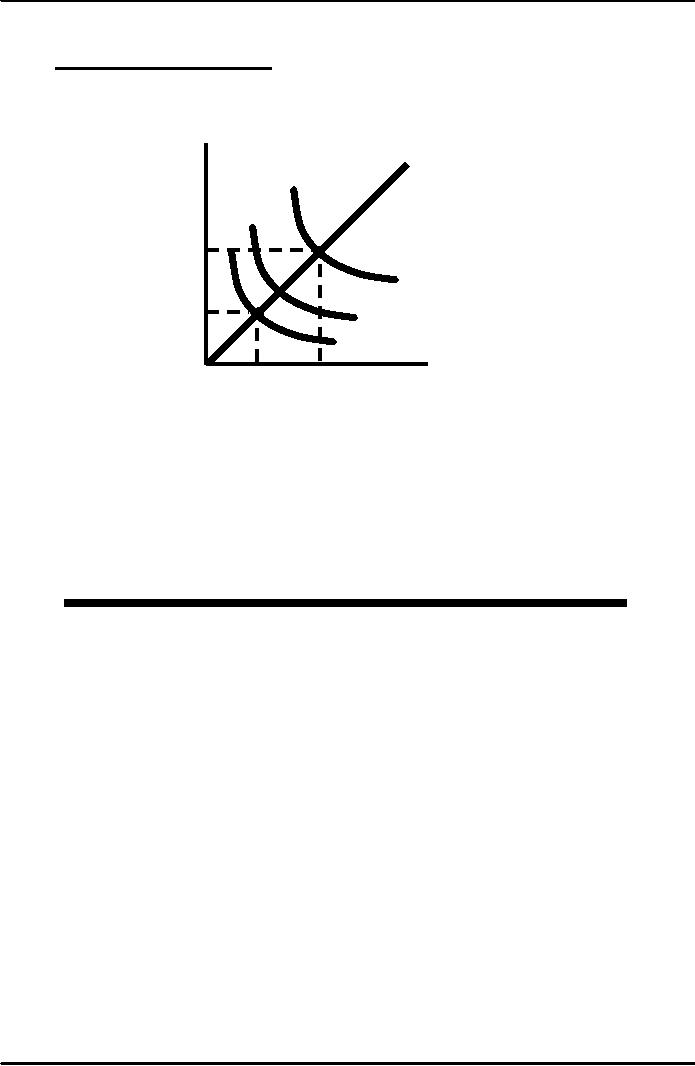
2.
Constant returns to scale:
output
doubles when all inputs
are doubled.
·
Size does
not affect
productivity
·
May have a
large number of
producers
·
Isoquants are
equidistant apart
Capital
(machine
hours)
A
Decreasing
returns to scale: output
less than doubles when
all inputs are
doubled
6
30
Constant
Returns:
4
Isoquants
are
20
equally spaced
2
10
Labor
(hours)
0
5
10
15
89
Microeconomics
ECO402
VU
3.
Decreasing returns to scale:
output
less than doubles when
all inputs are
doubled
·
Decreasing
efficiency with large
size
·
Reduction of
entrepreneurial abilities
·
Isoquants
become farther apart
A
Capital
(machine
hours)
Decreasing
Returns:
Isoquants
get further
apart
4
30
2
20
10
Labor
(hours)
0
5
10
Returns
to Scale in the Carpet
Industry
The
carpet industry has grown
from a small industry to a
large industry with some
very large
firms.
Question
Can the
growth be explained by the
presence of economies to
scale?
The
U.S. Carpet
Industry
Carpet
Shipments, 1996
(Millions
of Dollars per
Year)
1.
Shaw Industries
$3,202
6.
World Carpets
$475
2.
Mohawk Industries
1,795
7.
Burlington Industries
450
3.
Beaulieu of America
1,006
8.
Collins & Aikman
418
4.
Interface Flooring
820
9.
Masland Industries
380
5.
Queen Carpet
775
10.
Dixied Yarns
280
Are
there economies of
scale?
Costs (percent
of cost)
·
Capital --
77%
·
Labor --
23%
Large
Manufacturers
Increased in
machinery & labor
Doubling
inputs has more than
doubled output
Economies of
scale exist for large
producers
Small
Manufacturers
Small
increases in scale have
little or no impact on
output
Proportional
increases in inputs increase
output proportionally
90

Microeconomics
ECO402
VU
Constant returns
to scale for small
producers
91
Table of Contents:
- ECONOMICS:Themes of Microeconomics, Theories and Models
- Economics: Another Perspective, Factors of Production
- REAL VERSUS NOMINAL PRICES:SUPPLY AND DEMAND, The Demand Curve
- Changes in Market Equilibrium:Market for College Education
- Elasticities of supply and demand:The Demand for Gasoline
- Consumer Behavior:Consumer Preferences, Indifference curves
- CONSUMER PREFERENCES:Budget Constraints, Consumer Choice
- Note it is repeated:Consumer Preferences, Revealed Preferences
- MARGINAL UTILITY AND CONSUMER CHOICE:COST-OF-LIVING INDEXES
- Review of Consumer Equilibrium:INDIVIDUAL DEMAND, An Inferior Good
- Income & Substitution Effects:Determining the Market Demand Curve
- The Aggregate Demand For Wheat:NETWORK EXTERNALITIES
- Describing Risk:Unequal Probability Outcomes
- PREFERENCES TOWARD RISK:Risk Premium, Indifference Curve
- PREFERENCES TOWARD RISK:Reducing Risk, The Demand for Risky Assets
- The Technology of Production:Production Function for Food
- Production with Two Variable Inputs:Returns to Scale
- Measuring Cost: Which Costs Matter?:Cost in the Short Run
- A Firms Short-Run Costs ($):The Effect of Effluent Fees on Firms Input Choices
- Cost in the Long Run:Long-Run Cost with Economies & Diseconomies of Scale
- Production with Two Outputs--Economies of Scope:Cubic Cost Function
- Perfectly Competitive Markets:Choosing Output in Short Run
- A Competitive Firm Incurring Losses:Industry Supply in Short Run
- Elasticity of Market Supply:Producer Surplus for a Market
- Elasticity of Market Supply:Long-Run Competitive Equilibrium
- Elasticity of Market Supply:The Industrys Long-Run Supply Curve
- Elasticity of Market Supply:Welfare loss if price is held below market-clearing level
- Price Supports:Supply Restrictions, Import Quotas and Tariffs
- The Sugar Quota:The Impact of a Tax or Subsidy, Subsidy
- Perfect Competition:Total, Marginal, and Average Revenue
- Perfect Competition:Effect of Excise Tax on Monopolist
- Monopoly:Elasticity of Demand and Price Markup, Sources of Monopoly Power
- The Social Costs of Monopoly Power:Price Regulation, Monopsony
- Monopsony Power:Pricing With Market Power, Capturing Consumer Surplus
- Monopsony Power:THE ECONOMICS OF COUPONS AND REBATES
- Airline Fares:Elasticities of Demand for Air Travel, The Two-Part Tariff
- Bundling:Consumption Decisions When Products are Bundled
- Bundling:Mixed Versus Pure Bundling, Effects of Advertising
- MONOPOLISTIC COMPETITION:Monopolistic Competition in the Market for Colas and Coffee
- OLIGOPOLY:Duopoly Example, Price Competition
- Competition Versus Collusion:The Prisoners Dilemma, Implications of the Prisoners
- COMPETITIVE FACTOR MARKETS:Marginal Revenue Product
- Competitive Factor Markets:The Demand for Jet Fuel
- Equilibrium in a Competitive Factor Market:Labor Market Equilibrium
- Factor Markets with Monopoly Power:Monopoly Power of Sellers of Labor