Need for Speed: Parallelism: Scalability, Terminology, Parallelization OLTP Vs DSS

<< Total DQM: TDQM in a DWH, Data Quality Management Process

Need for Speed: Hardware Techniques: Data Parallelism Concept >>

Lecture-24

Need for Speed: Parallelism

Data warehouses often contain large tables and require techniques both for managing these large

tables and for providing good query performance across these large tables.

Parallel execution dramatically reduces response time for data-intensive operations on large

databases typically associated with Decision Support Systems (DSS) and data warehouses. You

can also implement parallel execution on certain types of online transaction processing (OLTP)

and hybrid systems.

Parallel execution is sometimes called parallelism. Simply expressed, parallelism is the idea of

breaking down a task so that, instead of one process doing all of the work in a query, many

processes do part of the work at the same time. An example of this is when four processes handle

four different quarters in a year instead of one process handling all four quarters by itself. The

improvement in performance can be quite high. In this case, data corresponding to each quarter

will be a partition, a smaller and more manageable unit of an index or table.

When to parallelize?

Useful for operations that access significant amounts of data.

Useful for operations that can be implemented independent of each other "Divide-&-Conquer"

Parallel execution improves processing for:

Large table scans and joins

Size

Creation of large indexes

Size

Partitioned index scans

D&C

Bulk inserts, updates, and deletes

Aggregations and copying

Size

D&C

Every operation can not be parallelized, there are some preconditions and one of them being that

the operations to be parallelized can be implemented independent of each other. This means that

there will be no interference between the operations while they are being parallelized. So what do

we gain out of parallelization; many things which can be divided into two such as with reference

to size and with reference to divide and conquer. Note that divide and conquer means that we

should be able to divide the problem and then solve it and then compile the results i.e. conquer.

For example in case of scanning a large table every row has to be checked, in such a case this can

be done in parallel thus reducing the overall time. There can be and are many examples too.

188

Are you ready to parallelize?

Parallelism can be exploited, if there is...

Symmetric multi-processors (SMP), clusters, or Massively Parallel (MPP)

systems AND

Sufficient I/O bandwidth AND

Underutilized or intermittently used CPUs (for example, systems where CPU

usage is typically less than 30%) AND

Sufficient memory to support additional memory -intensive processes such as

sorts, hashing, and I/O buffers

Word of caution

Parallelism can reduce system performance on over-utilized systems or systems with small I/O

bandwidth.

One can not just get up and parallelize, there are certain hardware and software requirements

other than the nature of the problem itself. The first and the foremost being a multiprocessor

environment which could consist of a small number of high performance processors to large

number of not so fast machines. Then you need bandwidth to port data to those processors and

exchange data between them. There are other options too such as a grid of those machines in the

computer lab that are not working during the night or are idling running just screen savers and the

list goes on.

A word of caution: Parallelism when not observed or practices carefully can actually degrade the

performance, in case the system is over ut ilized and the law of diminishing returns sets in or there

is insufficient bandwidth and it actually becomes the bottleneck and chokes the system.

189

Scalability Size is NOT everything

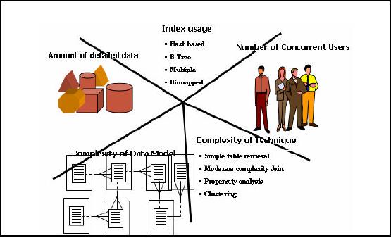
Figure-24.1: Size is NOT everything

It is common today for vendors and customers to boast about the size of their data warehouses.

And, in fact, size does matter. But it is not size alone as shown in Figure 24.1. Rather, significant

increases in data volume amplifies the issues associated with increasing numbers and varieties of

users, greater complexity and richness in the data model, and increasingly sophisticated and

complex business questions. Scalability is also about providing great flexibility and analysis

potential through richer, albeit more complex, data schemas. Finally, it is just as important to

allow for the increasing sophistication of the data warehouse users and evolving business needs.

Although the initial use of many data warehouses involves simple, canned, batch reporting many

companies are rapidly evolving to far more complex, ad hoc, iterative (not repetitive) business

questions "any query, any time" or "query freedom".

190

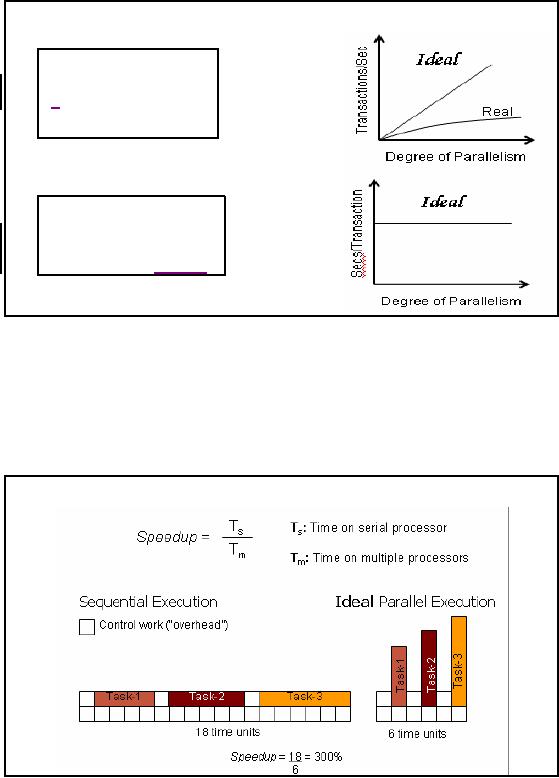
Scalability- Terminology

Speed-Up

More resources means

proportionally less time

for given amount of data.

Scale-Up

If resources increased in

proportion to increase in

data size, time is constant

Figure-24.2: Scalabilit y- Terminology

Its time for a reality check. It seems that increasing the processing power in terms of adding more

processors or computing resources should give a corresponding speedup are not correct. Ideally

this should be true, but in reality the entire problem is hardly parallelizable, hence the speedup is

non-linear. Similar behavior is experienced when the resources are increased in proportions to the

increase in problem size so that the time for a transaction remains same, ideally this is true, but

the reality is different. Why these things happen will become clear when we discuss Amdahl's

Law.

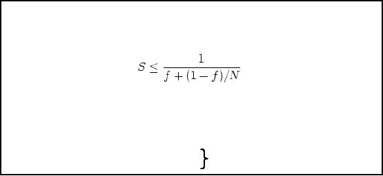
Quantifying Speed-up

Figure-24.3: Quantifying Speed-up

191

Data dependencies between different phases of computation introduce synchroniza tion

requirements that force sequential execution. Moreover, there is a wide range of capabilities

available in commercially implemented software in regard to the level of granularity at which

parallelism can be exploited.

As shown in figures 24.2 and 24.3, , the goal of ideal parallel execution is to completely

parallelize those parts of a computation that are not constrained by data dependencies. The

smaller the portion of the program that must be executed sequentially (s), the greater the

scalability of the computation.

Speed-Up & Amdahl's Law

Reveals maximum expected speedup from parallel algorithms given the proportion of task that

must be computed sequentially. It gives the speedup S as

f is the fraction of the problem that must be computed sequentially

N is the number of processors

As f approaches 0, S approaches N

Not

Example-1: f = 5% and N = 100 then S = 16.8

1:1

Example-2: f = 10% and N = 200 then S = 9.56

Ratio

The processing for parallel tasks can be spread across multiple processors. So, if 90% of our

processing can be parallelized and 10% must be serial we can speed up the process by a factor of

3.08 when we use four independent processors for the parallel portion. This example also

assumes 0 overhead and "perfect" parallelism. Thus, a database query that would run for 10

minutes when processed serially would, in this example, run in 2.63 minutes (10/3.08) when the

parallel tasks were executed on four independent processors.

As you can see, if we increase the overhead for parallel processing or decrease the amount of

parallelism available to the processors, the time it takes to complete the query will increase

according to the formula above.

192

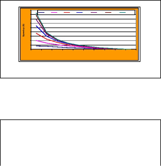
Amdahl's Law: Limits of parallelization

N=2

N=4

N=8

N=16

N=32

N=64

N=128

0.1

0.2

0.3

0.4

0.5

0.6

0.7

0.8

0.9

% sequential code (f)

For less

than

80% parallelism, the speedup drastically drops.

At 90% parallelism, 128 processors give performance of less than 10 processors.

Figure-24.4: Amdahl's Law

As we can see in the graphical representation of Amdahl's Law as shown in Figure24.4, the

realized benefit of additional proc essors is significantly diminishes as the amount of sequential

processing increases. In this graph, the vertical axis is the system speed-up. As the overall

percentage of sequential processing increases (with a corresponding decrease in parallel

processing) the relative effectiveness (utilization) of additional processors decreases. At some

point, the cost of an additional processor actually exceeds the incremental benefit.

Parallelization OLTP Vs. DSS

There is a big difference.

DSS

Parallelization of a SINGLE query

OLTP

Parallelization of MULTIPLE queries

Or Batch updates in parallel

During business hours, most OLTP systems should probably not use parallel execution. During

off-hours, however, parallel execution can effectively process high -volume batch operations. For

example, a bank can use parallelized batch programs to perform the millions of updates required

to apply interest to accounts.

The most common example of using parallel execution is for DSS. Complex queries, such as

those involving joins or searches of very large tables, are often best run in parallel.

193

Brief Intro to Parallel Processing

Parallel Hardware Architectures

§ Symmetric Multi Processing (SMP)

§ Distributed Memory or Massively Parallel Processing (MPP)

§ Non-uniform Memo ry Access (NUMA)

Parallel Software Architectures

§ Shared Memory

Shared everything

§ Shard Disk

§ Shared Nothing

Types of parallelism

§ Data Parallelism

§ Spatial Parallelism

NUMA

Usually on an SMP system, all memory beyond the caches costs an equal amount to reach for

each CPU. In NUMA systems, some memory can be accessed more quickly than other parts, and

thus called as Non -Uniform Memory Access. This term is generally used to describe a shared -

memory computer containing a hierarchy of memories, with different access times for each level

in the hierarchy. The distinguishing feature is that the time required to access memory locations is

not uniform i.e. access times to different locations can be different.

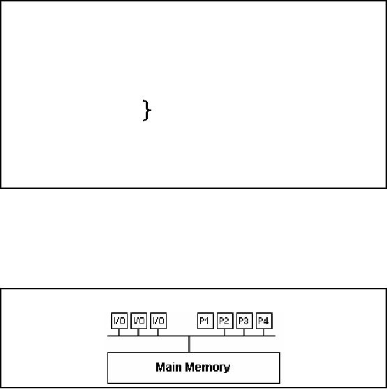
Symmetrical Multi Processing (SMP)

Figure-24.5: Symmetrical Multi Processing

SMP (Symmetric Multiprocessing) is a computer architecture that provides fast performance by

making multiple CPUs available to complete individual processes simultaneously

(multiprocessing). Unlike asymmetrical processing, any idle processor can be assigned any task,

and additional CPUs can be added to improve performance and handle increased work load. A

variety of specialized operating systems and hardware arrangements are available to support

SMP. Specific applications can benefit from SMP if the code allows multithreading.

SMP uses a single operating system and shares common memory and disk input/output resources.

Both UNIX and Windows NT support SMP.

194

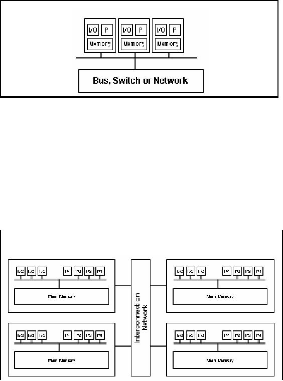
Distributed Memory Machines

Figure-24.6: Distributed Memory Machines

Special-purpose multiprocessing hardware comes in two flavors i.e. shared memory and

distributed memory machines. In a shared-memory machine, all processors have access to a

common main memory. In a distributed-memory machine, each processor has its own main

memory, and the processors are connected through a sophisticated interconnection network. A

collection of networked PCs is also a kind of distributed-memory parallel machine.

Communication between processors is an important prerequisite for all but the most trivial

parallel processing tasks (thus bandwidth can become a bottleneck). In a shared -memory

machine, a processor can simply write a value into a particular memory location, and all other

processors can read this value. In a distributed-memory machine, exchanging values of variables

involves explicit communication over the network, thus need for a high speed interconnection

network.

Distributed Shared Memory Machines

A little bit of both worlds!

It is also known as Virtual Shared Memory. This memory model is the attempt of a compromise

between shared und distributed memory. The distributed memory has been combined with an OS-

195

based message passing system which simulates the presence of a global shared memory, e.g.,

KSR: ''Sea of addresses'' and SGI: ''Interconnection fabric''. The plus side is that a sequential code

will r n immediately on that memory model. If the algorithms take advantage of the local

properties of data (i.e., most data accesses of a process can be served from its own local memory)

then a good scalability will be achieved.

Figure-24.7: Distributed Shared Memory Machines

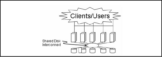
Shared disk RDBMS Architecture

Figure-24.7: Shared disk RDBMS Architecture

Shared disk database architecture as shown in Figure 24.7 is used by major database vendors. The

idea here is that all processors have equal access to data stored on disk. It does not mater if it is a

local disk or a remote disk, it is treated a single logical disk all the time. So we rely on high

bandwidth inter-processing communication to ship disk blocks to the requesting processor. This

approach allows multiple instances to see the same data. Every database instance sees everything.

Note that database instances mean different things for different databases. When I say database

instances in this context, it means collection of processes and threads that all share the same

database buffer cash. In the shared disk approach, transactions running on any instance can

directly read or modify any part of the database. Such systems require the use of inter-node

communication to synchronize update activities performed from multiple nodes. When two or

more nodes contend for the same data block, the node that has a lock on the data has to act on the

data and release the lock, before the other nodes can access the same data block.

Advantages:

A benefit of the shared disk approach is it provides a high level of fault tolerance with all data

remaining accessible even if there is only one surviving node.

Disadvantages:

Maintaining locking consistency over all nodes can become a problem in large clusters. So I can

have multiple database instances each with it's own database buffer cache all accessing the same

set of disk blocks. This is a shared everything disk architecture. Now if multiple database

instances are accessing the same tables and same blocks, th en some locking mechanism will be

required to maintain database buffer cash coherency. Because if a data block is in the buffer

cache of P1 and the same data block is in the buffer cash of P2 then there is a problem. So there is

something called distributed lock management that has to be implemented to maintain coherency

between the databases buffer cashes across these different database instances.

196

And that leads to a lot of performance issues in shared everything databases because every time

when lock management is performed, it becomes serial processing. There are two approaches to

solving this problem i.e. hardware mechanism and a software mechanism. In the hardware

mechanism, a coupling facility is used. The coupling facility manages all the locks to control

coherency in the database buffer cash. Another vendor took a different approach; because it sells

a more portable database that runs on any platform, therefore, it couldn't rely on special

hardware. Therefore, there is a software lock management system called the distributed lock

manager, which is used to mange across different database instances. In most cases both

techniques must guarantee that there is never incoherency of data blocks across database

instances.

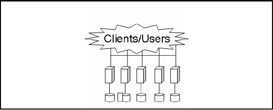
Shared Nothing RDBMS Architecture

Figure-24.8: Shared Nothing RDBMS Architecture

In case of shared nothing architecture as shown in Figure 24.8, there is no lock contention and

therefore any time you have locking problem then you also have serialization issue. The idea is

that each database table partition in the database instances e.g. the customer table and Order table

exist on all the database instances. So the parallelism is really already built in. There is never any

confusion and there is never any locking problem. If we join two tables with the same partitioning

column, and the partitioning was performed using hash partitioning, then that is a local join and is

very efficient.

A request will be made to the "owning" database instance to send the desired columns

(projection) from qualifying rows of the source table when data is required by one database

instance that is partitioned to a different database instance. In the function shipping approach, the

column and row filtering is performed locally by the "owning " database instance so that the

amount of information communicated to requesting database instance is only what is required.

This is different than in shared disk database architectures where full data blocks (no filtering) are

shipped to the requesting d atabase instance.

Advantages:

This works fine in environments where the data ownership by nodes changes relatively

infrequently. The typical reasons for changes in ownership are either database reorganizations or

node failures.

There is no overhead of maintaining data locking across the cluster

197

Disadvantages

The data availability depends on the status of the nodes. Should all but one system fail, then only

a small subset of the data is available.

Data partitioning is a way of dividing your tables etc. across multiple servers according to some

set of rules. However, this requires a good understanding of the application and its data access

patterns (which may change).

Shared disk Vs. Shared Nothing RDBMS

Important note: Do not confuse RDBMS architecture with hardware architecture.

Shared nothing databases can run on shared everything (SMP or NUMA) hardware.

Shared disk databases can run on shared nothing (MPP) hardware.

Now a very important point here is not to confuse the software architecture with the hardware

architecture. And there is lots of confusion on that point. People think that shared nothing

database architectures can only be implemented on shared nothing hardware architectures, that's

not true. People think that shared everything database architectures can only be implemented on

shared everything hardware architecture, which is not true either. So for example shared nothing

database like Teradata can work on an SMP machine, that's not a problem. Because the software

is shared nothing that does not mean that the hardware has to be shared nothing. SMP is

symmetric multi processing, shared memory, shared bus structure, shared I/O system and so on, it

is not a problem. In fact Informix is a shared nothing database architecture which was ori ginally

implemented on a shared everything hardware architecture which is an SMP machine.

So shared disk databases some times called shared everything databases are also run on shared

nothing hardware. Oracle is a shared everything database architecture and the original

implementation of the parallel query feature was written on machine called the N-Cube machine.

N-Cube machine is an MPP machine that is a shared nothing hardware architecture but that has a

shared everything database. In order to do that, a special layer of software called the VSD

(Virtual shared disk) is used. So when an I/O request is made, in a shared everything database

environment like ORACLE, every instance of the database can see every data block. If it is a

shared nothing environment how do I see other data blocks? With a basically an I/O device driver

which looks at the I/O request and if it is local, it says ok access it locally, if it is remote, it ships

the I/O request to another Oracle instance it does the I/O for me and then it ships the data back.

198

Shared Nothing RDBMS & Partitioning

Shared nothing RDBMS architecture requires a static partitioning of each table in the database.

How do you perform the partitioning?

Hash partitioning

Key range partitioning.

Lis t partitioning.

Round-Robin

Combinations (Range-Hash & Range-List)

Range partitioning maps data to partitions based on ranges of partition key values that you

establish for each partition. It is the most common type of partitioning and is often used with

dates. For example, you might want to partition sales data into monthly partitions.

Most shared nothing RDBMS products use a hashing function to define the static partitions

because this technique will yield an even distribution of data as long as the hashing key is

relatively well distributed for the table to be partitioned. Hash partitioning maps data to partitions

based on a hashing algorithm that database product applies to a partitioning key identified by the

DBA. The hashing algorithm evenly distributes rows among partitions, giving partitions

approximately the same size. Hash partitioning is the ideal method for distributing data evenly

across devices. Hash partitioning is a good and easy-to-use alternative to range partitioning when

data is not historical and there is no obvious column or column list where logical range partition

pruning can be advantageous.

List partitioning enables you to explicitly control how rows map to partitions. You do this by

specifying a list of discrete values for the partitioning column in the description for each partition.

This is different from range partitioning, where a range of values is associated with a partition

and with hash partitioning, where you have no control of the row-to-partition mapping. The

advantage of list partitioning is that you can group and organize unordered and unrelated sets of

data in a natural way.

Round robin is just like distributing a deck of cards, such that each player gets almost the same

number of cards. Hence it is "fair".

199

Table of Contents: