 |
Measures of Performance SRC Features and Instruction Formats |
| << Foundations of Computer Architecture, RISC and CISC |
| ISA, Instruction Formats, Coding and Hand Assembly >> |

Advanced Computer
Architecture-CS501
Lecture
Handout
Computer
Architecture
Lecture
No. 3
Reading
Material
Vincent
P. Heuring&Harry F. Jordan
Chapter2,
Chapter 3
Computer
Systems Design and Architecture
2.3,
2.4, 3.1
Summary
1)
Measures of
performance
2)
Introduction
to an example processor SRC
3)
SRC:Notation
4)
SRC
features and instruction
formats
Measures of
performance:
Performance
testing
To test or compare
the performance of machines,
programs can be run and
their
execution
times can be measured. However, the
execution speed may depend
on the
particular
program being run, and
matching it exactly to the
actual needs of the
customer
can be
quite complex. To overcome
this problem, standard programs
called "benchmark
programs"
have been devised. These programs
are intended to approximate
the real
workload
that the user will want to
run on the machine. Actual
execution time can be
measured
by running the program on
the machines.
Commonly
used measures of
performance
The
basic measure of performance of a
machine is time. Some
commonly used
measures
of this
time, used for comparison of
the performance of various
machines, are
·
Execution time
·
MIPS
·
MFLOPS
·
Whetstones
·
Dhrystones
·
SPEC
Execution
time
Execution
time is simply the time it
takes a processor to execute a
given program. The
time it
takes for a particular
program depends on a number of
factors other than
the
performance
of the CPU, most of which
are ignored in this measure. These
factors
include
waits for I/O, instruction
fetch times, pipeline
delays, etc.
The
execution time of a program
with respect to the processor, is
defined as
Execution
Time = IC x CPI x T
Page
42
Last
Modified: 01-Nov-06
Advanced Computer
Architecture-CS501
Where,
IC =
instruction count
CPI =
average number of system
clock periods to execute an
instruction
T =
clock period
Strictly
speaking, (IC×CPI)
should be the sum of the
clock periods needed to
execute
each
instruction. The manufacturers
for each instruction in the
instruction set
usually
provide
such information. Using the
average is a simplification.
MIPS
(Millions of Instructions per
Second)
Another
measure of performance is the
millions of instructions that
are executed by the
processor
per second. It is defined as
MIPS =
IC/ (ET x 106)
This
measure is not a very accurate
basis for comparison of
different processors. This
is
because
of the architectural differences of
the machines; some machines
will require
more
instructions to perform the
same job as compared to other
machines. For
example,
RISC
machines have simpler
instructions, so the same
job will require more
instructions.
This
measure of performance was popular in
the late 70s and early
80s when the VAX
11/780
was treated as a reference.
MFLOPS
(Millions of Floating Point
Instructions per
Second)
For
computation intensive applications,
the floating-point instruction
execution is a better
measure
than the simple
instructions. The measure
MFLOPS was devised with this
in
mind.
This measure has two
advantages over MIPS:
· Floating
point operations are
complex, and therefore, provide a
better picture of
the
hardware capabilities on which
they are run
· Overheads
(operand fetch from memory,
result storage to the
memory, etc.) are
effectively
lumped with the floating
point operations they
support
Whetstones
Whetstone
is the first benchmark
program developed specifically as a
benchmark
program
for performance measurement.
Named after the Whetstone
Algol compiler, this
benchmark
program was developed by using
the statistics collected
during the compiler
development.
It was originally an Algol program,
but it has been ported to
FORTRAN,
Pascal
and C. This benchmark has
been specifically designed to test
floating point
instructions.
The performance is stated in
MWIPS (millions of Whetstone
instructions per
second).
Dhrystones
Developed
in 1984, this is a small
benchmark program to measure
the integer
instruction
performance
of processors, as opposed to the
Whetstone's emphasis on floating
point
instructions.
It is a very small program,
about a hundred high-level-language
statements,
and
compiles to about 1~ 1½ kilobytes of
code.
Disadvantages
of using Whetstones and
Dhrystones
Both
Whetstones and Dhrystones are
now considered obsolete because of the
following
reasons.
· Small,
fit in cache
· Obsolete
instruction mix
· Prone to
compiler tricks
· Difficult
to reproduce results
· Uncontrolled
source code
We should
note that both the
Whetstone and Dhrystone benchmarks
are small programs,
which
encourage `over-optimization', and can be used
with optimizing compilers
to
distort
results.
Page
43
Last
Modified: 01-Nov-06
Advanced Computer
Architecture-CS501
SPEC
SPEC,
System Performance Evaluation
Cooperative, is an association of a number
of
computer
companies to define standard benchmarks
for fair evaluation and
comparison of
different
processors. The standard SPEC
benchmark suite
includes:
· A
compiler
· A
Boolean minimization
program
· A
spreadsheet program
· A
number of other programs
that stress arithmetic processing
speed
The
latest version of these
benchmarks is SPEC
CPU2000.
Advantages
· It
provides for ease of
publication.
· Each
benchmark carries the same
weight.
· SPEC
ratio is dimensionless.
· It is
not unduly influenced by
long running
programs.
· It is
relatively immune to performance
variation on individual
benchmarks.
· It
provides a consistent and fair
metric.
An
example computer: the SRC:
"simple RISC
computer"
An
example machine is introduced here to
facilitate our understanding of
various design
steps and
concepts in computer architecture. This
example machine is quite
simple, and
leaves
out a lot of details of a
real machine, yet it is
complex enough to illustrate
the
fundamentals.
SRC
Introduction
Attributes
of the SRC
·
The SRC contains 32 General
Purpose Registers: R0, R1, ...,
R31; each register is
of size
32-bits.
·
Two special purpose registers are
included: Program Counter
(PC) and Instruction
Register
(IR)
·
Memory word size is 32
bits
·
Memory space size is 232 bytes
·
Memory organization is 232 x 8 bits, this means
that the memory is byte
aligned
·
Memory is accessed in 32 bit
words ( i.e., 4 byte
chunks)
·
Big-endian byte storage is
used
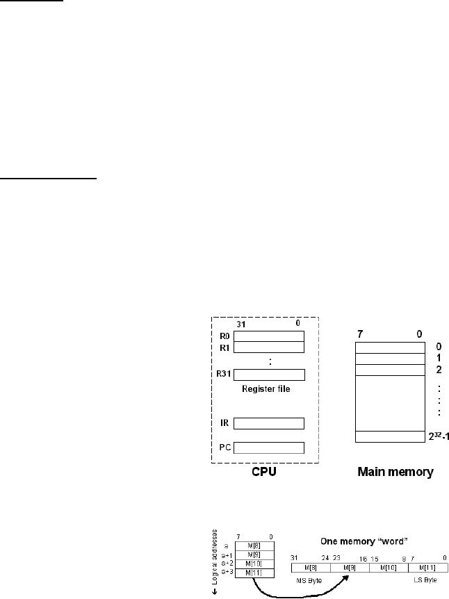
Programmer's
View of the
SRC
The
figure shows the attributes
of the
SRC;
the 32 ,32-bit registers that
are a
part of
the CPU, the two
additional
CPU
registers (PC & IR), and the
main
memory
which is 232
1-byte
cells.
SRC
Notation
We
examine the notation used
for the
SRC with
the help of some
examples.
·
R[3] means contents of
register
3 (R for
register)
· M[8]
means contents of memory
location 8 (M for
memory)
· A
memory word at address 8
is
defined
as the 32 bits at
address
Page
44
Last
Modified: 01-Nov-06
Advanced Computer
Architecture-CS501
8,9,10
and 11 in the memory. This is
shown in the figure.
· A special
notation for 32-bit memory
words is
M[8]<31...0>:=M[8]M[9]M[10]M[11]
is used
for concatenation.
Some
more SRC
Attributes
· All
instructions are 32 bits
long (i.e., instruction size is 1
word)
· All ALU
instructions have three
operands
·
The only way to access
memory is through load and store
operations
·
Only a few addressing
modes are supported
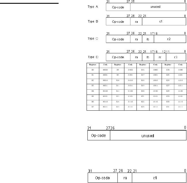
SRC:
Instruction Formats
Four
types of instructions
are
supported
by the SRC.
Their
representation
is given in the
figure
shown.
Before
discussing these
instruction
types in
detail, we take a look at
the
encoding
of general purpose registers
(the
ra, rb and rc fields).
Encoding
of the General Purpose
Registers
The
encoding for the general
purpose
registers is
shown in the table; it
will
be used
in place of ra, rb and rc in the
instruction
formats shown above.
Note
that
this is a simple 5 bit
encoding. ra,
rb and rc
are names of fields used
as
"place-holders",
and can represent any
one
of
these 32
registers. An
exception
is rb = 0; it does not mean the register
R0, rather it means no operand.
This will
be
explained in the following
discussion.
Type
A
Type
A is used for
only two
instructions:
· No
operation or nop, for which
the op-code = 0. This is useful in
pipelining
· Stop
operation stop, the op-code is 31
for this instruction.
Both of
these instructions do not
need an operand (are 0-operand
instructions).
Type
B
Type
B format includes
three
instructions;
all three use
relative
addressing
mode. These are
· The
ldr instruction, used to
load register from memory
using a relative
address.
(op-code
= 2).
o Example:
ldr
R3, 56
This
instruction will load the
register R3 with the
contents of the
memory
location
M [PC+56]
· The
lar instruction, for loading
a register with relative
address (op-code = 6)
Page
45
Last
Modified: 01-Nov-06
Advanced Computer
Architecture-CS501
o Example:
lar
R3, 56
This
instruction will load the
register R3 with the
relative address
itself
(PC+56).
· The
str is used to store register to
memory using relative
address (op-code = 4)
o Example:
str
R8, 34
This
instruction will store the register R8
contents to the memory
location
M
[PC+34]
The
effective address is computed at
run-time by adding a constant to
the PC. This
makes
the
instructions `re-locatable'.
Type
C
Type C
format has three
load/store
instructions,
plus
three
ALU
instructions.
These load/ store instructions
are
· ld,
the load register from
memory instruction (op-code =
1)
o Example
1:
ld R3,
56
This
instruction will load the
register R3 with the
contents of the
memory
location
M [56]; the rb field is 0 in
this instruction, i.e., it is
not used. This
is an
example of direct addressing
mode.
o Example
2:
ld R3,
56(R5)
The
contents of the memory
location M [56+R [5]] are
loaded to the
register
R3; the rb field ≠ 0. This
is an instance of indexed
addressing
mode.
· la is
the instruction to load a
register with an immediate
data value (which can
be
an
address) (op-code = 5 )
o Example1:
la R3,
56
The
register R3 is loaded with the
immediate value 56. This is
an instance
of
immediate addressing mode.
o Example
2:
la R3,
56(R5)
The
register R3 is loaded with the
indexed address 56+R [5].
This is an
example
of indexed addressing mode.
· The
st instruction is used to store register
contents to memory (op-code =
3)
o Example
1:
st R8,
34
This is
the direct addressing mode;
the contents of register R8 (R
[8]) are
stored to
the memory location M
[34]
o Example
2:
st R8,
34(R6)
An
instance of indexed addressing mode, M
[34+R [6]] stores the
contents
of R8(R
[8])
The ALU
instructions are
· addi,
immediate 2's complement
addition (op-code =
13)
o Example:
Page
46
Last
Modified: 01-Nov-06
Advanced Computer
Architecture-CS501
addi R3,
R4, 56
R[3]
R[4]+56
(rb
field = R4)
· andi,
the instruction to obtain
immediate logical AND,
(op-code = 42 )
o Example:
andi
R3, R4, 56
R3 is loaded
with the immediate logical
AND of the contents of
register
R4 and
56(constant value)
· ori,
the instruction to obtain
immediate logical OR (op-code = 23
)
o Example:
ori
R3, R4, 56
R3 is loaded
with the immediate logical
OR of the contents of register
R4
and
56(constant value)
Note:
1. Since
the constant c2 field is 17
bits,
For
direct addressing mode, only
the first 216 bytes of memory can
be
accessed (or the last
216 bytes if c2 is
negative)
In case
of the la instruction, only
constants with magnitudes
less
than
±216 can be loaded
During
address calculation using
c2, sign extension to 32
bits must
be
performed before the
addition
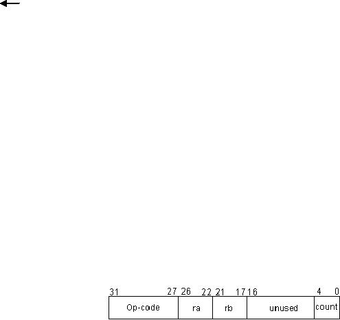
2. Type C
instructions, with some
modifications, may also be used
for
shift
instructions. Note
the
modification in the
following
figure.
The
four shift instructions
are
· shr
is the instruction used to
shift the bits right by
using value in (5-bit)
c3
field(shift
count)
· (op-code
= 26)
o Example:
shr
R3, R4, 7
shift R4
right 7 times in to R3.
Immediate addressing mode is
used.
· shra,
arithmetic shift right by
using value in c3 field
(op-code = 27)
o Example:
shra R3,
R4, 7
This
instruction has the effect
of shift R4 right 7 times in to
R3. Immediate
addressing
mode is used.
· The
shl instruction is for shift
left by using value in
(5-bit) c3 field (op-code =
28)
o Example:
shl
R8, R5, 6
shift R5
left 6 times in to R8.
Immediate addressing mode is
used.
· shc,
shift left circular by using
value in c3 field (op-code =
29)
o Example:
shc R3,
R4, 3
shift R4
circular 3 times in to R3.
Immediate addressing mode is
used.
Page
47
Last
Modified: 01-Nov-06
Table of Contents:
- Computer Architecture, Organization and Design
- Foundations of Computer Architecture, RISC and CISC
- Measures of Performance SRC Features and Instruction Formats
- ISA, Instruction Formats, Coding and Hand Assembly
- Reverse Assembly, SRC in the form of RTL
- RTL to Describe the SRC, Register Transfer using Digital Logic Circuits
- Thinking Process for ISA Design
- Introduction to the ISA of the FALCON-A and Examples
- Behavioral Register Transfer Language for FALCON-A, The EAGLE
- The FALCON-E, Instruction Set Architecture Comparison
- CISC microprocessor:The Motorola MC68000, RISC Architecture:The SPARC
- Design Process, Uni-Bus implementation for the SRC, Structural RTL for the SRC instructions
- Structural RTL Description of the SRC and FALCON-A
- External FALCON-A CPU Interface
- Logic Design for the Uni-bus SRC, Control Signals Generation in SRC
- Control Unit, 2-Bus Implementation of the SRC Data Path
- 3-bus implementation for the SRC, Machine Exceptions, Reset
- SRC Exception Processing Mechanism, Pipelining, Pipeline Design
- Adapting SRC instructions for Pipelined, Control Signals
- SRC, RTL, Data Dependence Distance, Forwarding, Compiler Solution to Hazards
- Data Forwarding Hardware, Superscalar, VLIW Architecture
- Microprogramming, General Microcoded Controller, Horizontal and Vertical Schemes
- I/O Subsystems, Components, Memory Mapped vs Isolated, Serial and Parallel Transfers
- Designing Parallel Input Output Ports, SAD, NUXI, Address Decoder , Delay Interval
- Designing a Parallel Input Port, Memory Mapped Input Output Ports, wrap around, Data Bus Multiplexing
- Programmed Input Output for FALCON-A and SRC
- Programmed Input Output Driver for SRC, Input Output
- Comparison of Interrupt driven Input Output and Polling
- Preparing source files for FALSIM, FALCON-A assembly language techniques
- Nested Interrupts, Interrupt Mask, DMA
- Direct Memory Access - DMA
- Semiconductor Memory vs Hard Disk, Mechanical Delays and Flash Memory
- Hard Drive Technologies
- Arithmetic Logic Shift Unit - ALSU, Radix Conversion, Fixed Point Numbers
- Overflow, Implementations of the adder, Unsigned and Signed Multiplication
- NxN Crossbar Design for Barrel Rotator, IEEE Floating-Point, Addition, Subtraction, Multiplication, Division
- CPU to Memory Interface, Static RAM, One two Dimensional Memory Cells, Matrix and Tree Decoders
- Memory Modules, Read Only Memory, ROM, Cache
- Cache Organization and Functions, Cache Controller Logic, Cache Strategies
- Virtual Memory Organization
- DRAM, Pipelining, Pre-charging and Parallelism, Hit Rate and Miss Rate, Access Time, Cache
- Performance of I/O Subsystems, Server Utilization, Asynchronous I/O and operating system
- Difference between distributed computing and computer networks
- Physical Media, Shared Medium, Switched Medium, Network Topologies, Seven-layer OSI Model