Join Techniques: Nested loop, Sort Merge, Hash based join

<< Special Indexing Techniques: Inverted, Bit map, Cluster, Join indexes

Data mining (DM): Knowledge Discovery in Databases KDD >>

Lecture- 28

Join Techniques

Background

Used to retrieve data from multiple tables.

Joins used frequently, hence lot of work on improving or optimizing them.

Simplest join that works in most cases is nested-loop join but results in quadratic time

complexity.

Tables identified by FROM clause and condition by WHERE clause.

Will cover different types of joins.

Join commands are statements that retrieve data from multiple tables. A join is identified by

multiple tables in the FROM clause, and the relationship between the tables to be joined is

established through the existence of a join condition in the WHERE clause. Because joins are so

frequently used in relational queries and because joins are so expensive, lot of effort has gone into

developing efficient join algorithms and techniques. The simplest i.e. nested-loop join is

applicable in all cases, but results in quadratic performance. Several fast join algorithms have

been developed and extensively used; these can be categorized as sort -merge, hash-based, and

index-based algorithms. In this lecture we will be covering the following join

algorithms/techniques:

Nested loop join

Sort Merge Join

Hash based join

Etc.

About Nested-Loop Join

Typically used in OLTP environment.

Limited application for DSS and VLDB

In DSS environment we deal with VLDB and large sets of data.

Traditionally Nested -Loop join has been and is used in OLTP environments, but for many

reasons, such a join mechanism is not suitable for VLDB and DSS environments. Nested loop

joins are useful when small subsets of data are joined and if the join condition is an efficient way

of accessing the inner table. Despite these restrictions/limitations, we will begin our discussion

with the traditional join technique i.e. nested loop join, so that you can appreciate the benefits of

the join techniques typically used in a VLDB and DSS environment.

226

Nested-Loop Join: Code

FOR i = 1 to n DO BEGIN

N rows in T1

IF ith row of T1 qualifies THEN BEGIN

For j = 1 to m DO BEGIN

M rows in T2

IF the ith row of T1 matches to jth row of T2 on join key THEN BEGIN

IF the jth row of T2 qualifies THEN BEGIN

produce output row

END

Nested loop join wo rks like a nested loop used in a high level programming language, where each

value of the index of the outer loop is taken as a limit (or starting point or whatever applicable)

for the index of the inner loop, and corresponding actions are performed on the statement(s)

following the inner loop. So basically, if the outer loop executes R times and for each such

execution the inner loop executes S times, then the total cost or time complexity of the nested

loop is O(RS).

Nested-loop joins provide efficient access when tables are indexed on join columns. Furthermore,

in many small transactions, such as those affecting only a small set of rows, index nested loops

joins are far superior to both sort -merge joins and hash joins. A nested loop join involves the

following steps:

1. The optimizer determines the major table (i.e. Table_A) and designates it as the outer

table. Table_A is accessed once. If the outer table has no useful indexes, a full table scan

is performed. If an index can reduce I/O costs, the index is used to locate the rows.

2. The other table is designated as the inner table or Table_B. Table_B is accessed once for

each qualifying row (or touple) in Table_A.

3. For every row in the outer table, DBMS accesses all the rows in the inner table. The outer

loop is for every row in outer table and the inner loop is for every row in the inner table.

If 10 rows from Table_A match the conditions in the query, Table_B is accessed 10 times. If

Table_B has a useful index on the join column, it might require 5 I/Os to read the data block for

each scan, plus one I/O for each data block. Hence the total cost of accessing Table_B would be

60 logical I/Os.

227

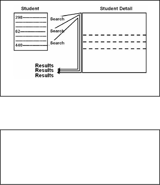
Nested-Loop Join: Working Example

For each qualifying row of Personal table,

Academic table is examined for matching rows.

Figure-28.1: The process of Nested-Loop Join without indexing

The process of creating the result set for a nested-loop join is achieved by nesting the tables, and

scanning the inner table repeatedly for each qualifying row of the outer table. This process is

shown in Figure-28.1: The question being asked is "What is the average GPS of undergraduate

male students?".

Nested-Loop Join: Order of Tables

If the outer loop executes R times and the inner loop executes S times, then the time complexity

will be O(RS).

The time complexity should be independent of the order of tables i.e. O(RS) is same as O(SR).

However, in the context of I/Os the order of tables does matter.

Along with this the relationship between the number of qualifyin g rows/blocks between the two

tables matters.

It is true that the actual number of matching rows returned as a result of the join would be

independent of the order of tables i.e. inner or outer; actually it is going to be even independent of

the type of join used. Now assume that depending on the filter criterion, different number of rows

is returned from the two tables to be joined. Let the rows returned from Table_A be RA and rows

returned from Table_B be RB, and let R A < RB. If Table_B would have been the outer table, then

for each row returned, the inner table i.e. Table_A would have been scanned (assuming no

indexing) RB times. However, if Table_A would have been the outer table, then for each row

returned, the inner table i.e. Table_B would have been scanned (assuming no indexing) RA times

228

i.e. less number of times scanned. Meaning, even if the inner table have fewer number of

qualifying rows, it is going to be scanned the number of times the qualifying rows of the outer

table. Hence the choice of tables does matter.

Nested-Loop Join: Cost Formula

Join cost = Cost of accessing Table_A +

# of qualifying rows in Table_A × Blocks of Table_B to be scanned for each qualifying row

Join cost = Blocks accessed for Table_A +

Blocks accessed for Table_A × Blocks accessed for Table_B

For a high level programming language, the time complexity of a nested -loop join remains

unchanged if the order of the loops are changed i.e. the inner and outer loops are interchanged.

However, this is NOT true for Nested-Loop-Joins in the context of DSS when we look at the I/O.

For a nested-loop join with two tables, the formula for estimating the join cost is:

Join cost = Cost of accessing Table_A +

# of qualifying rows in Table_A × Blocks of Table_B to be scanned for each qualifying row.

Join cost = Blocks accessed for Table_A +

Blocks accessed for Table_A × Blocks accessed for Table_B

For a Nested-Loop join inner and outer tables are determined as follows:

The outer table is usually the one that has:

The smallest number of qualifying rows, and/or

The largest numbers of I/Os required to locate the rows.

The inner table usually has:

The largest number of qualifying rows, and/or

The smallest number of reads required to locate rows.

229

Nested-Loop Join: Cost of reorder

Table_A = 500 blocks and

Table_B = 700 blocks.

Qualifying blocks for Table_A QB(A) = 50

Qualifying blocks for Table_B QB(B) = 100

Join cost A&B = 500 + 50× 700 = 35,500 I/Os

Join cost B&A = 700 + 100× 500 = 50,700 I/Os

i.e. an increase in I/O of about 43%.

For example, if qualifying blocks for Table_A QB(A) = 50 and qualifying blocks for Table_B

QB(B) = 100 and size of Table_A is 500 blocks and size of Table_B is 700 blocks then Join cost

A&B = 500 + 50× 700 = 35,500 I/Os and using the other order i.e. Table_B outer table and

Table_A as inner table, the join cost B&A = 700 + 100× 500 = 50,700 I/Os i.e. an increase in I/O

of about 43%.

Nested-Loop Join: Variants

1. Naive nested-loop join

2. Index nested-loop join

3. Temporary index nested-loop join

Working of Query optimizer

There are many variants of the traditional nested-loop join. The simplest case is when an entire

table is scanned; this is called a naive nested -loop join. If there is an index, and that index is

exploited, then it is called an index nested-loop join. If the index is built as part of the query plan

and subsequently dropped, it is called as a temporary index nested -loop join. All these variants

are considered by the query optimizer before selecting the most appropriate join

algorithm/technique.

Sort-Merge Join

Joined tables to be sorted as per WHERE clause of the join predicate.

Query optimizer scans for (cluster) index, if exists performs join.

In the absence of index, tables are sorted on the columns as per WHERE clause.

If multiple equalities in WHERE clause, some merge columns used.

230

The Sort -Merge join requires that both tables to be joined are sorted on those columns that are

identified by the equality in the WHERE clause of the join predicate. Subsequently the tables are

merged based on the join columns. The query optimizer typically scans an index on the columns

which are part of the join, if one exists on the proper set of columns, fine, else the tables are

sorted on the columns to be joined , resulting in what is called a cluster index. However, in rare

cases, there may be multiple equalities in the WHERE clause, in such a case, the merge columns

are taken from only some of the given equality clauses.

Because each table is sorted, the Sort -Merge Join operator gets a row from each table and

compares it one at a time with the rows of the other table. For example, for equi-join operations,

the rows are returned if they match/equal on the join predicate. If they are not equal or don't

match, whic hever row has the lower value is discarded, and next row is obtained from that table.

This process is repeated until all the rows have been exhausted.

The Sort -Merge join process just described works as follows:

· Sort Table_A and Table_B on the join column in ascending order, then scan them to do a

``merge'' (on join column), and output result tuples/rows.

Proceed with scanning of Table_A until current A_tuple ≤ current B_tuple, then

proceed scanning of Table_B until current B_tuple ≤ current A_tuple; do this

until current A_tuple = current B_tuple.

At this point, all A_tuples with same value in Ai (current A_group) and all

B_tuples with same value in Bj (current B_group) match; output <a, b> for all

pairs of such tuples/records.

Update pointers, resume scanning Table_A and Table_B .

· Table_A is scanned once; each B group is scanned once per matching Table_A tuple.

(Multiple scans of a B group are likely to find needed pages in buffer.)

· Cost: M log M + N log N + (M+N)

§ The cost of scanning is M+N, could be M*N (very unlikely!)

231

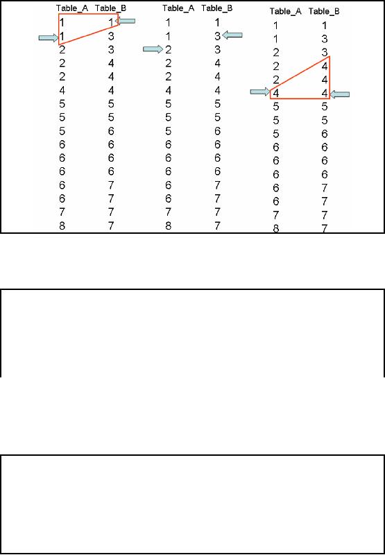
Figure-28.2: The process of merging

Fig-28.2 shows the process of merging two sorted tables with IDs shown. Conceptually the

merging is similar to the merging you must have studies in Merge_Sort in your Algorithm course.

Sort-Merge Join: Note

Very fast.

Sorting can be expensive.

Presorted data can be obtained from existing B-tree.

Sort-Merge join itself is very fast, but it can be an expensive choice if sort operations are required

frequently i.e. the contents of the t able's change often resulting in deterioration of the sort order.

However, it may so happen that even if the data volume is large the desired data can be obtained

presorted from existing B-tree. For such a case sort -merge join is often the fastest availabl e join

algorithm.

Hash-Based Join: Working

Suitable for the VLDB environment.

The choice which table first gets hashed plays a pivotal role in the overall performance of the join

operation, this decided by the optimizer.

The joined rows are identified by collisions i.e. collisions are "good" in case of hash join.

232

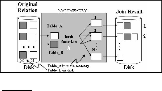
Hash joins are suitable for the VLDB environment as they are useful for joining large data sets or

tables. The choice about which table first gets hashed plays a pivotal role in the overall

performance of the join operation, and left to the optimizer. The optimizer decides by using the

smaller of the two tables (say) Table_A or data sources to build a hash table in the main memory

on the join key used in the WHERE clause. It then scans the larger table (say) Table_B and probes

the hashed table to find the joined rows. The joined rows are identified by collisions i.e. collisions

are "good" in case of hash join.

The optimizer uses a hash join to join two tables if they are joined using an equij oin and if either

of the following conditions are true:

A large amount of data needs to be joined.

A large portion of the table needs to be joined.

This method is best used when the smaller table fits in the available main memory. The cost is

then limited to a single read pass over the data for the two tables. Else the "smaller" table has to

be partitioned which results in unnecessary delays and degradation of performance due to

undesirable I/Os.

Figure-28.3: Working of Hash-based join

Cost of Hash -Join

· In partitioning phase, read + write both operations requires 2(M+N) I/Os.

· In matching phase, read both requires M+N I/Os.

233

Hash-Based Join: Large "small" Table

Smaller of the two tables may grow too big to fit into the main memory.

Optimizer performs partitioning, but is not simple.

Multi-step approach followed, each step has a build phase and probe phase.

Both tables entirely consumed and partitioned via hashing.

Hashing guarantees any two joining records will fall in same pair of partitions.

Task reduced to multiple, but smaller, instances of the same tasks.

It may so happen that the smaller of the two tables grows too big to fit into the main memory,

then the optimizer breaks it up by partitioning, such that a partition can fit in the main memory.

However, it is not that simple because the qualifying rows of both the tables have to fall in the

corresponding partition pairs that are hashed (build) and probed. Thus in such a case the hash join

proceeds in several steps. Each step has a build phase and probe phase. Initially, the two tables

are entirely consumed and partitioned (using a hash function on the hash keys) into multiple

partitions. The number of such partitions is sometimes called the partitioning fan -out. Using the

hash function on the hash keys (based on the predicates in the WHERE clause) guarantees that any

two joining records must be in the same pair of partitions. Therefore, the task of joining two large

tables gets reduced to multiple, but smaller, instances of the same tasks. The hash join is then

applied to each pair of partitions.

Hash-Based Join: Partition Skew

Partition skew can become a problem.

Hashing works under the assumption of uniformity of data distribution, may not be always true.

Consequently hash-based join degrades into nested-loop join.

Solution: Make available other hash functions to be chosen by the optimizer; that better distribute

the input.

Partition skew can become a problem in hash-join. In the first step of hash join, records are

hashed into the main memory into their corresponding bucket. This being done based on the hash

function used. However, an attribute being hashed may not be uniformly distributed within the

relation, and some buckets may then contain more records than other buckets. When this

difference becomes large, the corresponding bucket may no longer fit in the main memory. As a

consequence, hash -based join degrades into performance of a nested-loop join. The only possible

solution is to make available other hash functions to be chosen by the optimizer; that better

distribute the input.

234

Hash-Based Join: Intrinsic Skew

Intrinsic skew can become a problem for hash, as well as sort -merge join.

The skew is in data, NOT due to hash function.

Example: Many non-CS majors registering for CS-101 instead of CS students in summer.

Intrinsic skew occurs when attributes are not distributed uniformly; it is also called attribute value

skew. For example a basic Computer Science (CS) course being offered in summer, and taken by

many non -CS majors who want to know about computers. The course taken by few CS-majors

who missed it or got an incomplete (i.e. I) grade during the regular semester due to one reason or

another. Ironically, intrinsic skew effects the performance of both hash and sort -merge joins.

Sort-merge join works best when the join attributes are the primary key of both tables. This

property guarantees absence of duplicates, so that a record in the left -hand-side of the relation

will join with at most one record in the right -hand-side of the relation, thus avoiding the intrinsic

skew.

235

Table of Contents: