Inventory Control:INVENTORY COSTS, INVENTORY MODELS (E.O.Q. MODELS)

<< PERT / CPM:Exercises

Inventory Control:Purchasing model with shortages >>

Operations Research (MTH601)

3-5

4-5

Resource availability:

Number of operators = 50

Equipments X = 1, Y = 1, Z = 1

Segment III: Inventory Control

Lectures 11 -16

Operations Research (MTH601)

INVENTORY AND CONTROL

Inventory is the physical stock of items held in any business for the purpose of future production

or sales. In a production shop the inventory may be in the form of raw materials. When the items

are in production process, we have the inventory as in-process inventory and at the end of the

production cycle inventory is in the form of finished goods. We shall be dealing only with the

finished goods inventory. The problem of determining inventory policies is not a new concept

beginning. It is only in he last two decades that it has been tackled with quantitative techniques

and mathematical models, a method amenable to optimization.

Inventory planning is the determination of the type and quantity of inventory items that would be required at

future points for maintaining production schedules. Inventory planning is generally based on information from the past

and also on factors that would arise in future. Once this sort of planning is over, the control process starts, which

means that actual and planned inventory positions are compared and necessary action taken so that the business

process can function efficiently.

In inventory control, we are primarily concerned with the inventory cost control. The aim is focussed to

bring down the total inventory cost per annum as much as possible. Two important questions are (1) how much to

stock or how much to buy and (2) how often to buy or when to buy. An answer to the above questions is usually

given by certain mathematical models, popularly known as `economic order quantity models' or `economic lot/batch

size models (E.O.Q.).'

INVENTORY COSTS

There are four major elements of inventory costs that should be taken for analysis, such as

Item cost, Rs. C1/item.

(1)

(2)

Ordering cost, Rs. C2/order.

Holding cost Rs. C3/item/unit time.

(3)

(4)

Shortage cost Rs. C4/item/Unit time.

Item Cost (C1)

This is the cost of the item whether it is manufactured or purchased. If it is manufactured, it includes such

items as direct material and labour, indirect materials and labour and overhead expenses. When the item is

purchased, the item cost is the purchase price of 1 unit. Let it be denoted by Rs. C1 per item.

Purchasing or Setup or Acquisition or Ordering Cost (C2)

Administrative and clerical costs are involved in processing a purchase order, expediting, follow up etc., It

includes transportation costs also. When a unit is manufactured, the unit set up cost includes the cost of labour and

materials used in the set up and set up testing and training costs. This is denoted by Rs. C2 per set up or per order.

Inventory holding cost (C3)

Operations Research (MTH601)

If the item is held in stock, the cost involved is the item carrying or holding cost. Some of the costs included

in the unit holding cost are

(1)

Taxes on inventories,

(2)

Insurance costs for inflammable and explosive items,

(3)

Obsolescence,

(4)

Deterioration of quality, theft, spillage and damage to times,

(5)

Cost of maintaining inventory records.

This cost is denoted by Rs. C3/item/unit time. The unit of time may be days, months, weeks or years.

Shortage Cost (C4)

The shortage cost is due to the delay in satisfying demand (due to wrong planning); but the demand is

eventually satisfied after a period of time. Shortage cost is not considered as the opportunity cost or cost of lost sales.

The unit shortage cost includes such items as,

(1)

Overtime requirements due to shortage,

(2)

Clerical and administrative expenses.

(3)

Cost of expediting.

(4)

Loss of goodwill of customers due to delay.

(5)

Special handling or packaging costs.

(6)

Lost production time.

This cost is denoted by Rs. C4 per item per unit time of shortage.

INVENTORY MODELS (E.O.Q. MODELS)

The inventory control model can be broadly classified into two categories:

(1) Deterministic inventory problems.

(2) Probabilistic or stochastic inventory problems.

In the deterministic type of inventory control, the parameters like demand, ordering quantity cost, etc are

already known or have been ascertained and there is no uncertainty. In the stochastic inventory control, the uncertain

aspects are taken into account.

First let us consider the inventory control of the deterministic type. There are four EOQ models which are

discussed below. The first one is the well-known Wilson's inventory model.

Model 1: Purchasing model with no shortages: (Wilson's model)

The following assumptions are made in deriving the formula for economic order quantity.

(1)

Demand (D) is at a constant rate.

(2)

Replacement of items is instantaneous (lead time is zero).

(3)

The cost coefficients C1, C2, and C3 are constant.

There is no shortage cost or C4 = 0.

(4)

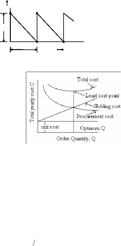
This mode represented graphically in fig. 1. This is also known as a saw tooth model (because of its shape).

Operations Research (MTH601)

Quantity

Q =Im

Time

Fig. 1

Fig. 2

In this model, at time t = 0, we order a quantity Q which is stored as maximum inventory, 1m. The time `t' denotes the

time of one period or it is the time between orders or it is the cycle time. During this time, the items are depleting and

reaching a zero value at the end of time t. At time t another order of the same quantity is to be placed to bring the

stock upto Q again and the cycle is repeated. Hence this is a fixed order quantity model.

The total cost for this model for one cycle is made up of three cost components.

Total cost/period = (Item cost + set up cost + holding cost/period)

Item cost per period = (Cost of item) × (number of items ordered/period)

= C1Q

(1)

Purchase or set up cost per period = C2 (only one set up per period)

Item holding cost per period = (Holding cost) × (average inventory per period) × (time per period)

= C3 Q 2 × t

(2)

Operations Research (MTH601)

Therefore the total cost per period (C ′) = C Q + C + C Q 2 × t

(3)

But the time for one period t = Q D

(4)

Therefore the total cost per unit time, C = C′ t

(5)

C + C1D + C2

(6)

3 2

Substituting the value of t, we get C = C D + C D Q + C Q 2

(7)

The cost components of the above equations can be represented as shown in fig 2 and an optimum order quantity for

one period is found when

Purchase cost = Item holding cost.

C2D C3Q

2C2D

Q2 =

Q* =

(8)

This minimum inventory cost per unit time can also be found by differentiating C with respect to Q and equating it to

zero. The derivative of the equation is,

dC -C2 D

(9)

Solving for Q, we get

2C2D

Q* =

(10)

This value of Q* is the economic order quantity and any other order quantity will result in a higher cost.

The corresponding period t* is found from

t* = Q* D

(11)

The optimum number of orders per year is determined from

N * = D Q*

where D is the demand per year.

Operations Research (MTH601)

Example 1: The demand rate for a particular item is 12000 units/year. The ordering cost is Rs. 100 per order and

the holding cost is Rs. 0.80 per item per month. If no shortages are allowed and the replacement is instantaneous,

determine:

(1)

The economic order quantity.

(2)

The time between orders.

(3)

The number of orders per year.

(4)

The optimum annual cost if the cost of item is Rs. 2 per item.

Solution: Note that the holding cost is given per month and convert the same into cost per

year.

C1 = Rs. 2/item

C2 = Rs. 100/order

C3 = Rs. 0.80/item/month

= Rs. 9.6/item/year

D = 12000 items/year

The economic order quantity

2C2 D

Q* =

2×100×12000

9.6

= 500 units

The time between orders

t* = Q* D = 500 / 12000 yr.

= 500 1000 month

= 0.5 month

The number of orders/year

N = D Q* = 12000 / 500 = 24

The optimum annual cost

Table of Contents: