GEOMETRIC MEAN:Number of Pupils, QUARTILE DEVIATION:

<< GEOMETRIC MEAN:HARMONIC MEAN, MID-QUARTILE RANGE

GEOMETRIC MEAN:MEAN DEVIATION FOR GROUPED DATA >>

MTH001 Elementary Mathematics

LECTURE # 27:

Concept of dispersion

Absolute and relative measures of dispersion

Range

Coefficient of dispersion

Quartile deviation

Coefficient of quartile deviation

Let us begin the concept of DISPERSION.

Just as variable series differ with respect to their location on the horizontal axis (having

different `average' values); similarly, they differ in terms of the amount of variability which

they exhibit.

Let us understand this point with the help of an example:

EXAMPLE:

In a technical college, it may well be the case that the ages of a group of first-year students

are quite consistent, e.g. 17, 18, 18, 19, 18, 19, 19, 18, 17, 18 and 18 years.

A class of evening students undertaking a course of study in their spare time may show just

the opposite situation, e.g. 35, 23, 19, 48, 32, 24, 29, 37, 58, 18, 21 and 30.

It is very clear from this example that the variation that exists between the various values of

a data-set is of substantial importance. We obviously need to be aware of the amount of

variability present in a data-set if we are to come to useful conclusions about the situation

under review. This is perhaps best seen from studying the two frequency distributions given

below:

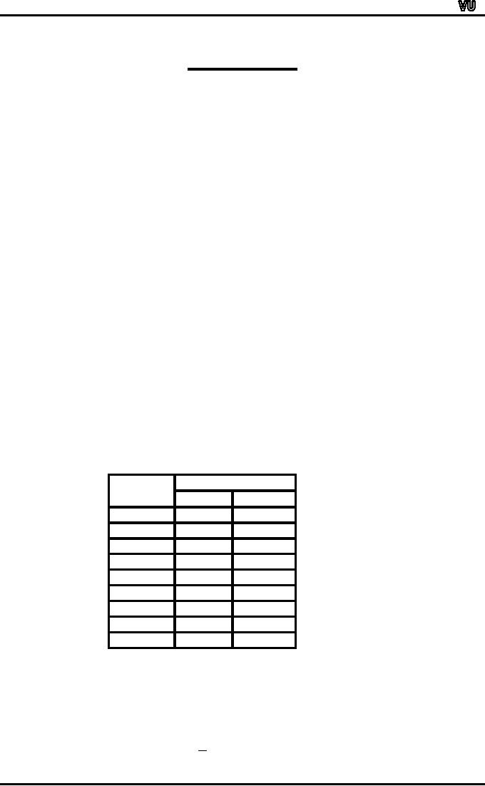
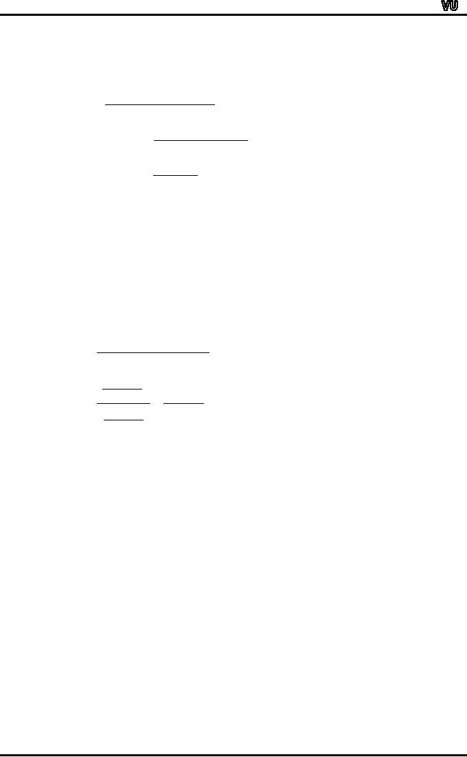
EXAMPLE:

The sizes of the classes in two comprehensive schools in different areas are as

follows:

Number

Number of Classes

of Pupils

Area A

Area B

10 14

15 19

20 24

25 29

30 34

35 39

40 44

45 - 49

If the arithmetic mean size of class is calculated, we discover that the answer is identical:

27.33 pupils in both areas.

Average class-size of each school

X = 27.33

Page

188

MTH001 Elementary Mathematics

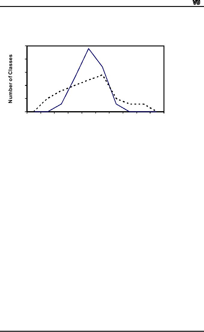
Even though these two distributions share a common average, it can readily be seen that

they are entirely DIFFERENT.

And the graphs of the two distributions (given below) clearly indicate this fact.

Area

1 0 2 5 2 0 3 5 3 0 4 4 -4 0 5

Number of Pupils

The question which must be posed and answered is `In what way can these two situations

be distinguished?'

We need a measure of variability or DISPERSION to accompany the relevant

measure of position or `average' used.

The word `relevant' is important here for we shall find one measure of dispersion

which expresses the scatter of values round the arithmetic mean, another the scatter of

values round the median, and so forth. Each measure of dispersion is associated with a

particular `average'.

Absolute versus Relative Measures of Dispersion:

There are two types of measurements of dispersion: absolute and relative.

An absolute measure of dispersion is one that measures the dispersion in terms of

the same units or in the square of units, as the units of the data.

For example, if the units of the data are rupees, meters, kilograms, etc., the units of

the measures of dispersion will also be rupees, meters, kilograms, etc.

On the other hand, relative measure of dispersion is one that is expressed in the

form of a ratio, co-efficient of percentage and is independent of the units of measurement.

A relative measure of dispersion is useful for comparison of data of different nature.

A measure of central tendency together with a measure of dispersion gives an adequate

description of data. We will be discussing FOUR measures of dispersion i.e. the range, the

quartile deviation, the mean deviation, and the standard deviation.

RANGE:

The range is defined as the difference between the two extreme values of a data-set,

i.e. R = Xm X0 where Xm represents the highest value and X0 the lowest.

Evidently, the calculation of the range is a simple question of MENTAL arithmetic.

The simplicity of the concept does not necessarily invalidate it, but in general it gives no idea

of the DISTRIBUTION of the observations between the two ends of the series. For this

reason it is used principally as a supplementary aid in the description of variable data, in

conjunction with other measures of dispersion. When the data are grouped into a frequency

distribution, the range is estimated by finding the difference between the upper boundary of

the highest class and the lower boundary of the lowest class.

Page

189

MTH001 Elementary Mathematics

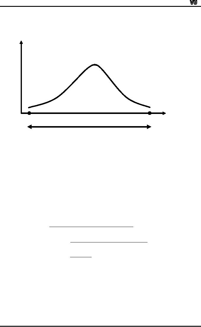
We now consider the graphical representation of the range:

Rang

Obviously, the greater the difference between the largest and the smallest values, the

greater will be the range. As stated earlier, the range is a simple concept and is easy to

compute. However, because of the fact that it is computed from only the two extreme values

in a data-set, it has two serious disadvantages.

1. It ignores all the INFORMATION available from the intermediate observations.

2. It might give a MISLEADING picture of the spread in the data.

From THIS point of view, it is an unsatisfactory measure of dispersion. However, it is

APPROPRIATELY used in statistical quality control charts of manufactured products, daily

temperatures, stock prices, etc.

It is interesting to note that the range can also be viewed in the following way:

It is twice of the arithmetic mean of the deviations of the smallest and largest values round

the mid-range i.e.

(Midrange - X0 ) + (X m - Midrange )

Midrange - X0 + X m - Midrange

X - X0

= m

Because of what has been just explained, the range can be regarded as that measure of

dispersion which is associated with the mid-range. As such, the range may be employed to

indicate dispersion when the mid-range has been adopted as the most appropriate average.

The range is an absolute measure of dispersion. Its relative measure is known as the CO-

EFFICIENT OF DISPERSION, and is defined by the relation given below:

Coefficient of Dispersion:

Page

190

MTH001 Elementary Mathematics

(Range)

Mid - Range

Xm - X0

X - X0

= m

Xm + X0

This is a pure (i.e. dimensionless) number and is used for the purposes of COMPARISON.

(This is so because a pure number can be compared with another pure number.)

For example, if the coefficient of dispersion for one data-set comes out to be 0.6

whereas the coefficient of dispersion for another data-set comes out to be 0.4, then it is

obvious that there is greater amount of dispersion in the first data-set as compared with the

second.

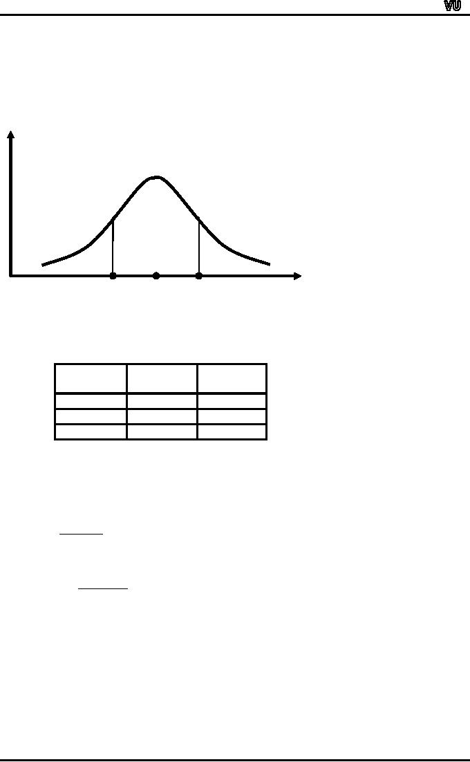
QUARTILE DEVIATION:

The quartile deviation is defined as half of the difference between the third and first

quartiles i.e.

Q3 - Q1

Q.D. =

It is also known as semi-interquartile range.

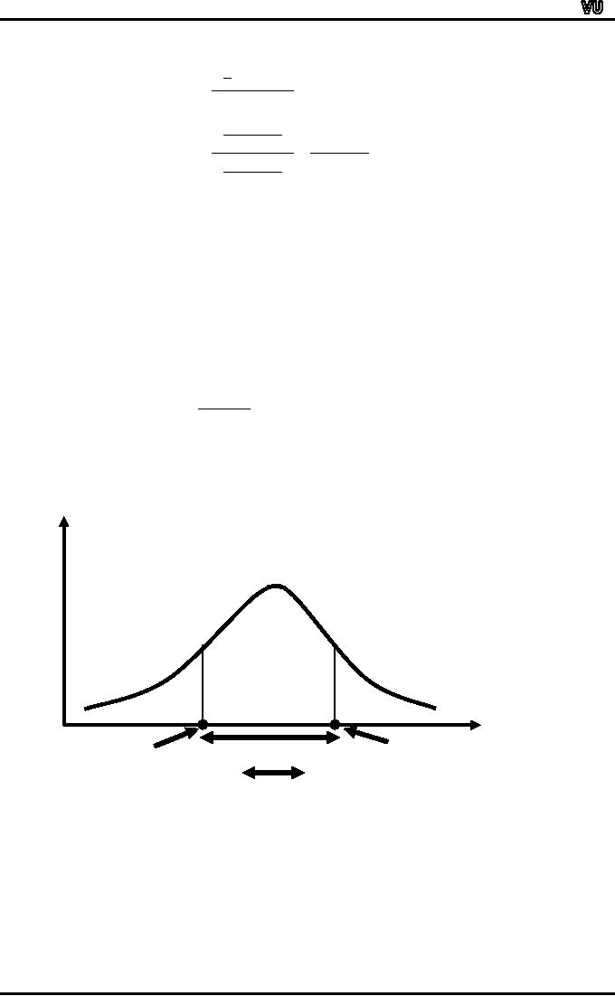
Let us now consider the graphical representation of the quartile deviation:

Inter-quartile

Quartile Deviation

(Semi Inter-quartile Range)

Although simple to compute, it is NOT an extremely satisfactory measure of dispersion

because it takes into account the spread of only two values of the variable round the

median, and this gives no idea of the rest of the dispersion within the distribution.

The quartile deviation has an attractive feature that the range "Median + Q.D."

contains approximately 50% of the data.

This is illustrated in the figure given below:

Page

191

MTH001 Elementary Mathematics

50%

Median-Q.D.

Median Median+Q.D.

Let us now apply the concept of quartile deviation to the following example:

EXAMPLE:

The shareholding structure of two companies is given below:

Company

1st quartile

60 shares

165 shares

Median

185 shares

3rd quartile

270 shares

210 shares

The quartile deviation for company X is

270 - 60

= 105

For company Y, it is

210 - 165

= 22

A comparison of the above two results indicate that there is a considerable concentration of

shareholders about the MEDIAN number of shares in company Y, whereas in company X,

there does not exist this kind of a concentration around the median. (In company X, there is

approximately the SAME numbers of small, medium and large shareholders.)

From the above example, it is obvious that the larger the quartile deviation, the

greater is the scatter of values within the series. The quartile deviation is superior to range

as it is not affected by extremely large or small observations. It is simple to understand and

easy to calculate.

The mean deviation can also be viewed in another way:

Page

192

MTH001 Elementary Mathematics

It is the arithmetic mean of the deviations of the first and third quartiles round the median i.e.

(M - Q1 ) + (Q3 - M )

M - Q1 + Q3 - M

Q - Q1

= 3

Because of what has been just explained, the quartile deviation is regarded as that measure

of dispersion which is associated with the median. As such, the quartile deviation should

always be employed to indicate dispersion when the median has been adopted as the most

appropriate average.

The quartile deviation is also an absolute measure of dispersion. Its relative measure called

the CO-EFFICIENT OF QUARTILE DEVIATION or of Semi-Inter-quartile Range, is defined

by the relation:

Coefficient of Quartile Deviation:

Quartile Deviation

Mid - Quartile Range

Q3 - Q1

Q - Q1

= 3

Q3 + Q1

The Coefficient of Quartile Deviation is a pure number and is used for COMPARING the

variation in two or more sets of data.

The next two measures of dispersion to be discussed are the Mean Deviation and the

Standard Deviation. In this regard, the first thing to note is that, whereas the range as well

as the quartile deviation are two such measures of dispersion which are NOT based on all

the values, the mean deviation and the standard deviation are two such measures of

dispersion that involve each and every data-value in their computation.

The range measures the dispersion of the data-set around the mid-range, whereas

the quartile deviation measures the dispersion of the data-set around the median.

How are we to decide upon the amount of dispersion round the arithmetic mean?

It would seem reasonable to compute the DISTANCE of each observed value in the series

from the arithmetic mean of the series.

But the problem is that the sum of the deviations of the values from the mean is

ZERO! (No matter what the amount of dispersion in a data-set is, this quantity will always be

zero, and hence it cannot be used to measure the dispersion in the data-set.)

Then, the question arises, `HOW will we be able to measure the dispersion present in our

data-set?'

In an attempt to answer this question, we might look at the numerical differences

between the mean and the data values WITHOUT considering whether these are positive or

negative. By ignoring the sign of the deviations we will achieve a NON-ZERO sum, and

Page

193

MTH001 Elementary Mathematics

averaging these absolute differences, again, we obtain a non-zero quantity which can be

used as a measure of dispersion. (The larger this quantity, the greater is the dispersion in

the data-set).

This quantity is known as the MEAN DEVIATION.

Let us denote these absolute differences

by `modulus of d'

or `mod d'. Then, the mean deviation is given by

MEAN DEVIATION:

∑| d |

M.D. =

As the absolute deviations of the observations from their mean are being averaged,

therefore the complete name of this measure is Mean Absolute Deviation --- but generally, it

is simply called "Mean Deviation". In the next lecture, this concept will be discussed in detail.

(The case of raw data as well as the case of grouped data will be considered.)Next, we will

discuss the most important and the most widely used measure of dispersion i.e. the

Standard Deviation.

Page

194

Table of Contents: