 |
Operations
Research (MTH601)
266
The
profit function
f4(s, x4) = p(x4) +
f3*(s-x3)
We
analyse all possible
combinations of investment with
the available capital and we
tabulate the net
returns
as shown below
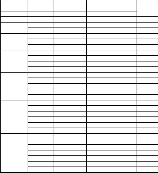
Capital,
s,
Allotment
Allotment
Net
Return from
x4*
for
A
for
B,C & D
all
ventures
s
= x2 +
x1
x4
(s-x4)
f4(s)
s=0
0
0
0
s=1
0
1
0
+ 6 = 6*
1
1
0
5+0=5
s=2
0
2
0+8=8
1
1
5
+ 6= 11*
0
2
0
6+0=6
s=3
0
3
0
+ 10 = 10
1
2
5
+ 8 = 13*
1
2
1
6
+ 6 = 12
3
0
7+0=7
s=4
0
4
0
+ 12 = 12
1
3
5
+ 10 = 15 *
1
2
2
6
+ 8 = 14
3
1
7
+ 6 = 13
4
0
8+0=8
s=5
0
5
0
+ 14 = 4
1
4
5
+ 12 = 17*
1
2
3
6
+ 10 = 16
3
2
7
+ 8 = 15
4
1
8
+ 6 = 14
5
0
8+0=8
s=6
0
6
0
+ 16 = 16
1
5
5
+ 14 = 19*
1
2
4
6
+ 12 = 18
3
3
7
+ 10 = 17
4
2
8
+ 8 = 16
5
1
8
+ 6 = 14
6
0
8+0=8
Analysis
of the Result
From
the above table with a total
capital of 6 units, we get
the maximum returns as Rs.
19. This is
achieved
by allotting one unit to
business A and the remaining
5 units to business ventures B, C
and D
combined.
Then referring to the
results of the three-stage solution we
have to allot either 3 units
to B or 4 units
to
B. Thus there are two
cases to consider.
266
Operations
Research (MTH601)
267
Case
1
If
we allot 3 units of capital to B,
then the remaining capital
is only 6 - (1+3) = 2 units,
that can be
allotted
to business ventures C and D.
Then from the results of
the two-stage problem, we
see the optimum
allotment
of one unit capital to C and
the remaining one unit to D
can be made. Therefore, for
this case, the
allotment
of capital to A, B, C and D are 1, 3, 1
and 1 units
respectively.
Case
2
If
we allot 4 units of capital to B,
then the remaining capital
is only 6-(1+4) = 1 unit
that can be allotted
to
business ventures C and D.
Then from the results of
the two-stage problem, we
see that the
optimum
allotment
of one unit of capital to C
and nothing to D. Hence for
this case, the allotments of
capital to A, B, C
and
D are 1, 4, 1 and 0
respectively.
Both
the policies yield the net
return of Rs. 19.
A
truck can carry a load of 10
tonnes of a product. There
are three types of products
to be
Example
transported
by the truck. The weights and profits
are as tabulated in the next
page. With the condition
that at
least
one of each type must be
transported, determine the
loading which will maximize
the total profit.
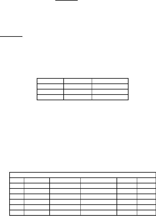
Type
Profit
(Rs.)
Weight
(Tonnes)
A
20
1
B
50
2
C
60
2
In
this problem, a decision is to be taken
as to how many units of A, B
and C should be
Solution:
transported.
Thus let each stage
represent transported. We divide the
problem into three stages.
The one stage
problem
is to divide the amount of
product C to be transported.
One
Stage Problem:
The
profit per unit of C (weight
= 2 tonnes) is Rs. 60. The
restriction is that at least
one unit of types A
and
B must be transported. Out of
maximum 10 tonnes, (1 + 2) tonnes
are allotted to A and B.
Hence we can
load
the remaining 7 tonnes only.
Let the total load be transported vary
from 2 tonnes to 7 tonnes
represented by
si. Let
xi be the states representing
one, two or three units (i =
1, 2, 3). Let f1*
represent the optimum profit
in
one
stage problem. The results
are as in the table
below.
xi
fi*
xi*
si
1
2
3
2
1
x 60 = 60
Not
feasible
Not
feasible
60
1
3
1
x 60 = 60
Not
feasible
Not
feasible
60
1
4
1
x 60 = 60
2
x 60 = 120
Not
feasible
120
2
5
1
x 60 = 60
2
x 60 = 120
Not
feasible
120
2
6
1
x 60 = 60
2
x 60 = 120
3
x 60 = 180
180
3
7
1
x 60 = 60
2
x 60 = 120
3
x 60 = 180
180
3
267
Operations
Research (MTH601)
268
Two
Stage Problem:
Here
the decision is taken as to
how much of product B and C
to be transported. We take the
decision
to
allot same space to
transport product B and the
remaining space is available
for C for which the
optimum
values
are taken from the
results of one stage
problem. The optimum values
are taken from the
results of one
stage
problem. The space to be
used for B and C together
varies from 4 tonnes to 9
tonnes.
Let
x2 represent
the amount of units if
product of type B to be transported.
Then the remaining (s2 -
x2)
tonnes
of space are available for
product C. The results are
as shown in the table
below.
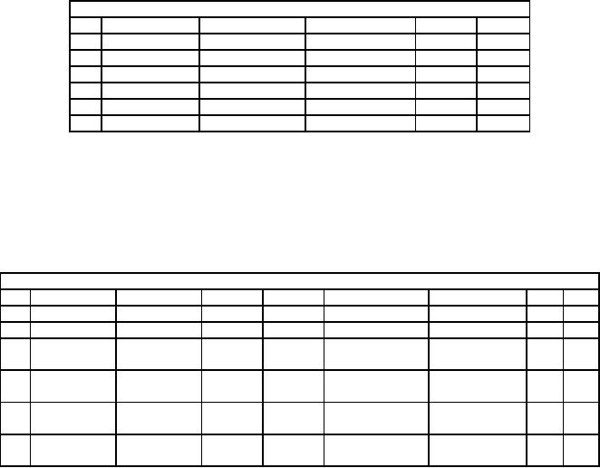
s2
x2
f2*
x2*
1
2
3
2
50+60=
110
Not
feasible
Not
feasible
110
1
3
50+60=
110
Not
feasible
Not
feasible
110
1
4
50+120=
170
100+60
= 160
Not
feasible
170
1
5
50+120=
170
100+60
= 160
Not
feasible
170
1
6
50+180=
230
100+120
= 220
150
+ 60 = 210
230
1
7
50+180=
230
100+120
= 220
150
+ 60 = 210
230
1
Three
Stage Problem:
Here
we consider all the three
types of products. Let s3 be the space available
for transporting items, x3
be
the amount of product of
type A to be transported, so that
(s3 - x3)
tonnes of space is available
for sending
products
B and C together for which
the optimum profit is taken
from the two stage
problem. The space
available
(s3)
varies from 5 tonnes to 10
tonnes and x3
varies
from one tonne to 6 tonnes.
The results of the
three
stage
problem are as shown in the
table below.
s3
x3
f3*
x3*
1
2
3
4
5
6
5
20+110=130
Not
feasible
-
-
-
-
130
1
6
20+110=130
40+110=150
N.F
-
-
-
150
2
7
20+170=190
40+110=150
60+110
-
-
-
190
1,3
=170
8
20+170=190
40+170=210
60+110
N.F
-
-
210
2
=170
9
20+230=250
40+110=210
60+130
80+110
-
-
250
1
=190
=190
10
20+230=250
40+230=270
60+170
80+170
100+110=210
120+110=250
270
2
=230
=250
268
Operations
Research (MTH601)
269
EXERCISES
1.
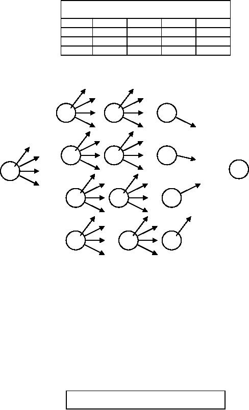
A
minimum distance pipe line
is to be constructed between points A
and E passing
successively
through
one node of each B, C an D as
shown in the figure on the next
page. The distances from A
to B and
from
D to E are shown in figure.
To
1
2
3
4
From
1
12
15
24
28
2
15
16
17
24
3
24
17
16
15
4
28
21
15
12
The
distances between B and C
and between C and D are
given in the table. Find
the solution through
dynamic
programming
1
1
1
2
2
2
3
3
3
4
4
4
2.
An
investor has Rs. 50000 to
invest. He has three
alternatives to choose. The
estimated returns for
different
amounts of capital invested in
each alternative are
tabulated. Zero allocation returns
Rs. 0. What is the
optimal
investment policy?
Amount
Alternative
(Rs.)
1
2
3
269
Table of Contents:
- Introduction:OR APPROACH TO PROBLEM SOLVING, Observation
- Introduction:Model Solution, Implementation of Results
- Introduction:USES OF OPERATIONS RESEARCH, Marketing, Personnel
- PERT / CPM:CONCEPT OF NETWORK, RULES FOR CONSTRUCTION OF NETWORK
- PERT / CPM:DUMMY ACTIVITIES, TO FIND THE CRITICAL PATH
- PERT / CPM:ALGORITHM FOR CRITICAL PATH, Free Slack
- PERT / CPM:Expected length of a critical path, Expected time and Critical path
- PERT / CPM:Expected time and Critical path
- PERT / CPM:RESOURCE SCHEDULING IN NETWORK
- PERT / CPM:Exercises
- Inventory Control:INVENTORY COSTS, INVENTORY MODELS (E.O.Q. MODELS)
- Inventory Control:Purchasing model with shortages
- Inventory Control:Manufacturing model with no shortages
- Inventory Control:Manufacturing model with shortages
- Inventory Control:ORDER QUANTITY WITH PRICE-BREAK
- Inventory Control:SOME DEFINITIONS, Computation of Safety Stock
- Linear Programming:Formulation of the Linear Programming Problem
- Linear Programming:Formulation of the Linear Programming Problem, Decision Variables
- Linear Programming:Model Constraints, Ingredients Mixing
- Linear Programming:VITAMIN CONTRIBUTION, Decision Variables
- Linear Programming:LINEAR PROGRAMMING PROBLEM
- Linear Programming:LIMITATIONS OF LINEAR PROGRAMMING
- Linear Programming:SOLUTION TO LINEAR PROGRAMMING PROBLEMS
- Linear Programming:SIMPLEX METHOD, Simplex Procedure
- Linear Programming:PRESENTATION IN TABULAR FORM - (SIMPLEX TABLE)
- Linear Programming:ARTIFICIAL VARIABLE TECHNIQUE
- Linear Programming:The Two Phase Method, First Iteration
- Linear Programming:VARIANTS OF THE SIMPLEX METHOD
- Linear Programming:Tie for the Leaving Basic Variable (Degeneracy)
- Linear Programming:Multiple or Alternative optimal Solutions
- Transportation Problems:TRANSPORTATION MODEL, Distribution centers
- Transportation Problems:FINDING AN INITIAL BASIC FEASIBLE SOLUTION
- Transportation Problems:MOVING TOWARDS OPTIMALITY
- Transportation Problems:DEGENERACY, Destination
- Transportation Problems:REVIEW QUESTIONS
- Assignment Problems:MATHEMATICAL FORMULATION OF THE PROBLEM
- Assignment Problems:SOLUTION OF AN ASSIGNMENT PROBLEM
- Queuing Theory:DEFINITION OF TERMS IN QUEUEING MODEL
- Queuing Theory:SINGLE-CHANNEL INFINITE-POPULATION MODEL
- Replacement Models:REPLACEMENT OF ITEMS WITH GRADUAL DETERIORATION
- Replacement Models:ITEMS DETERIORATING WITH TIME VALUE OF MONEY
- Dynamic Programming:FEATURES CHARECTERIZING DYNAMIC PROGRAMMING PROBLEMS
- Dynamic Programming:Analysis of the Result, One Stage Problem
- Miscellaneous:SEQUENCING, PROCESSING n JOBS THROUGH TWO MACHINES
- Miscellaneous:METHODS OF INTEGER PROGRAMMING SOLUTION