Dimensional Modeling DM: ER modeling, The Paradox, ER vs. DM,

<< ROLAP: Relational Database, ROLAP cube, Issues

Process of Dimensional Modeling: Four Step: Choose Business Process, Grain, Facts, Dimensions >>

Lecture-13

Dimensional Modeling (DM)

Relational modeling techniques are used to develop OLTP systems. A typical OLTP system

involves a very large number of focused queries i.e. accesses a small number of database rows,

which are accessed mostly via unique or primary keys using indexes. The relational model, with

well thought -out de-normalization, can result in a physical database design that meets the

requirements of OLTP systems. Decision support systems, however, involve fundamentally

different queries. These systems involve fewer queries that are usually not focused i.e. access

large percentages of the database tables, often performing joins on multiple tables and in many

cases aggregating and sorting the results. OLTP systems are NOT good at performing joins.

In the early days of DSS, OLTP systems were used for decision support with very large databases

and performance problems were encountered. Some surprising findings were the deterioration of

the performance of the DBMS optimizers when the number of tables joined exceeded a certain

threshold. This problem led to development of a second type of model that "flattened out" the

relational model structures by creating consolidated reference tables from several pre -joined

existing tables i.e. converting snow-flakes into stars.

However, according to one school of thought, DM should not be the first reaction, but followed

after trying indexing, and views and weighing different options carefully.

The need for ER modeling?

Problems with early COBOLian data processing systems.

Data redundancies.

From flat file to Table, each entity ultimately becomes a Table in the physical schema.

Simple O(n2) Join to work with Tables.

ER is a logical design technique that seeks to remove the redundancy in data. Imagine the

WAPDA line-man going from home to home and recording the meter reading from each

customer. In the early COBOLian days of computing (i.e. long before relational databases were

invented), this data was transferred into the computer from the original hand recordings as a

single file consisting of number of fields, such as name of customer, address, meter number, date,

time , current reading etc. Such a record could easily have been 500 bytes distributed across 10

fields. Other than the recording date and meter reading, EVERY other field was getting repeated.

Although having all of this redundant data in the computer was very useful, but had its down

sides too, from the aspect of storing and manipulating data. For example, data in this form was

difficult to keep consistent because each record stood on its own. The customer's name and

address appeared many times, because this d ata was repeated whenever a new reading was taken.

Inconsistencies in the data went unchecked, because all of the instances of the customer address

were independent, and updating the customer's address was a chaotic transaction as there are

literally a dozen ways to just represent "house no"!

Therefore, in the early days of COBOLian computing, it became evident (I guess first to Dr.

Codd) to separate out the redundant (or repeating) data into distinct tables, such as a customer

master table etc., but at a price. The then available systems for data retrieval and manipulation

became overly complex and inefficient because, this required careful attention to the processing

algorithms for linking these sets of tables together i.e. join operation. Note that a ty pical nested

loop join will run in O(n2) time if the two tables are separate such as customer and product bought

by the customers. This requirement resulted in database system that was very good at linking

tables, and paved the way for the relational datab ase revolution.

Why ER Modeling has been so successful?

Coupled with normalization drives out all the redundancy from the database.

Change (or add or delete) the data at just one point.

Can be used with indexing for very fast access.

Resulted in success of OLTP systems.

The ER modeling technique is a discipline used to highlight the microscopic relationships among

data elements or entities. The pinnacle of achievement of ER modeling is to remove all

redundancy from the data. This is enormously benefi cial for the OLTP systems, because

transactions are made very simple and deterministic i.e. no surprises in the overall query

execution time i.e. it must finish (say) under 5 seconds. The transaction for updating customer's

address gets reduced to a single record lookup in a customer address master table. This lookup is

controlled by a customer address key, which defines uniqueness of the customer address record

i.e. PK. This lookup is implemented using an index, hence is extremely fast. It can be stated

without hesitation, that the ER techniques have contributed to the success of the OLTP systems.

Need for DM: Un-answered Qs

Lets have a look at a typical ER data model first.

Some Observations:

§ All tables look-alike, as a consequence it is difficult to identify:

Which table is more important ?

Which is the largest?

Which tables contain numerical measurements of the business?

Which table contain nearly static descriptive attributes?

Is DM really needed? In order to better understand the need for DM lets have a look at the

diagram showing the retail data in simplified 3NF.

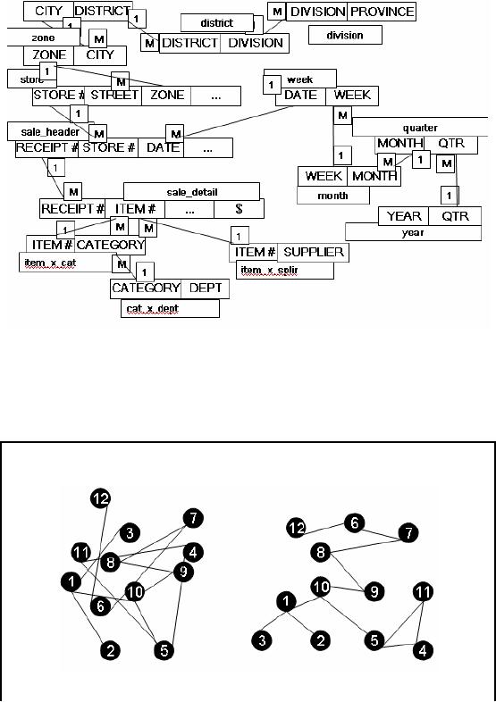
Having a close look at the diagram, it reveals that a separate table has been maintained to store

different entities resulting in a complex overall model. Probing the model to get informative

insight about data is not straightforward. For example, we can not tell by looking at the model the

relative importance of tables. We can not know the table sizes (though we can guess by looking at

just headers), and most importantly we can not tell about business dimensions by just looking at

the table headers i.e. which tables contain business measurements of the business , which tables

contain the static descriptive data and so on.

Many topologies for the same ER diagram, all appearing different.

§ Very hard to visualize and remember.

A large number of possible connections to any two (or more) tables

Figure-13.1: Need for DM: Un-answered Qs

Even for the simple retail example, there are more than a dozen tables that are linked together by

puzzling spaghetti of links; and this is just the beginning. This problem is further complicated by

the fact that there can be numerous (actually exponentially large) topologies for the same system

created by different people, and re-orienting makes them better (or worse).

The problem becomes even more complex for the ER model for an enterprise, which has

hundreds of logical entities, and for a high end ERP systems for a large multinational there could

be literally thousands of such entities. Each of these entities typically translates into a physical

table when the database is implemented. Making sense of this "mess" is almost impossible,

communicating it to someone even more difficult.

Need for DM: The Paradox

The Paradox: Trying to make information accessible using tables resulted in an inability

to query it efficiently!

ER and Normalization result in large number of tables which are:

§ Hard to understand by the users (DB programmers)

Hard to navigate optimally by DBMS software

Real value of ER is in using tables individually or in pairs

Too complex for queries that span multiple tables with a large number of records

However, there is a paradox! In the fervor to make OLTP systems fast and efficient, the designers

lost sight of the original, most important goal i.e. querying the databases to retrieve

data/information. Thus this defeats the purpose as follows:

Due to the sheer complexity of the ER graph, end users cannot understand or remember

an ER model, and as a consequence cannot navigate an ER model. There is no graphical

user interface (GUI) that takes a general ER model and makes it usable to end users,

because this tends to be an NP-Complete problem.

ER models are typically chaotic and "random", hence software cannot usefully query

them. Cost-based optimizers that attempt to do this are infamous for making the wrong

choices, and disastrous performance consequences.

And finally, use of the ER modeling technique defeats the basic attraction of data

warehousing, namely intuitive and high -performance retrieval of data.

ER vs. DM

Constituted to optimize DSS query

Constituted to optimize OLTP performance.

performance.

Models the macro relationships among data

Models the micro relationships among data

elements with an overall deterministic

elements.

strategy.

All dimensions serve as equal entry points to

A wild variability of the structure of ER models.

the fact table.

Very vulnerable to changes in the user's querying Changes in user querying habits can be catered

habits, because such schemas are asymmetrical. by automatic SQL generators.

Table 13.1: ER vs. DM

1- ER models are constituted to (a) remove redundancy from the data model, (b) facilitate

retrieval of individual records h aving certain critical identifiers, and (c) therefore, optimize On -

line Transaction Processing (OLTP) performance.

2- ER modeling does not really model a business; rather, it models the micro relationships among

data elements. ER modeling does not have "business rules," it has "data rules."

3- The wild variability of the structure of ER models means that each data warehouse needs

custom, handwritten and tuned SQL. It also means that each schema, once it is tuned, is very

vulnerable to changes in the user's querying habits, because such schemas are asymmetrical.

===============================================================

1-In DM, a model of tables and relations is constituted with the purpose of optimizing decision

support query performance in relational databases, relative to a measurement or set of

measurements of the outcome(s) of the business process being modeled.

2-Even a big suite of dimensional models has an overall deterministic strategy for evaluating

every possible query, even those crossing many fact tables.

3-All dimensions serve as equal entry points into the fact table. Changes in users' querying habits

don't change the structure of the SQL or the standard ways of measuring and controlling

performance.

How to simplify an ER data model?

Two general methods:

D e-Normalization

Dimensional Modeling (DM)

The shortcomings of ER modeling did not unnoticed. Since the beginning of the relational

database revolution, many DB designers tried to deliver the design data to end users as ra ther

look-alike "simpler designs with a "dimensional" i.e. ease of understanding and performance as

the highest goals. There are actually two ways of "simplifying" the ER model i.e. (i) De -

normalization and (ii) Dimensional Modeling.

What is DM?...

A simpler logical model optimized for decision support.

Inherently dimensional in nature, with a single central fact table and a set of smaller

dimensional tables.

Multi-part key for the fact table

Dimensional tables with a single-part PK.

Keys are usually system generated.

Results in a star like structure, called star schema or star join.

All relationships mandatory M-1.

Single path between any two levels.

Supports ROLAP operations.

DM is a logical design technique that seeks to present the data in a standard, instinctive structure

that supports high-performance and ease of understanding. It is inherently dimensional in nature,

and it does adhere to the relational model, but with some important restrictions. Such as, every

dimensional model is composed of one "central" table with a multipart key, called the fact table,

and a set of smaller tables called dimension tables. Each dimension table has a single-part

primary key that corresponds exactly to one of the components of the multipart key in the fact

table. This results in a characteristic "star -like" structure or star schema.

DM is a logical design technique that seeks to present the data in a standard, instinctive structure

that supports high-performance and ease of understanding. It is inherently dimensional in nature,

and it does adhere to the relational model, but with some important restrictions. Such as, every

dimensional model is composed of one "central" table with a multipart key, called the fact table,

and a set of smaller tables called dimension tables. Each dimension table has a single-part

primary key that corresponds exactly to one of the components of the multipart key in the fact

table. This results in a characteristic "star -like" structure or star schema.

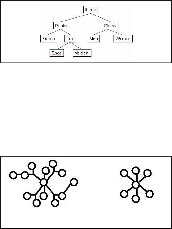
Dimensions have Hierarchies

Analysts tend to look at the data through dimension at a particular "level" in the hierarchy

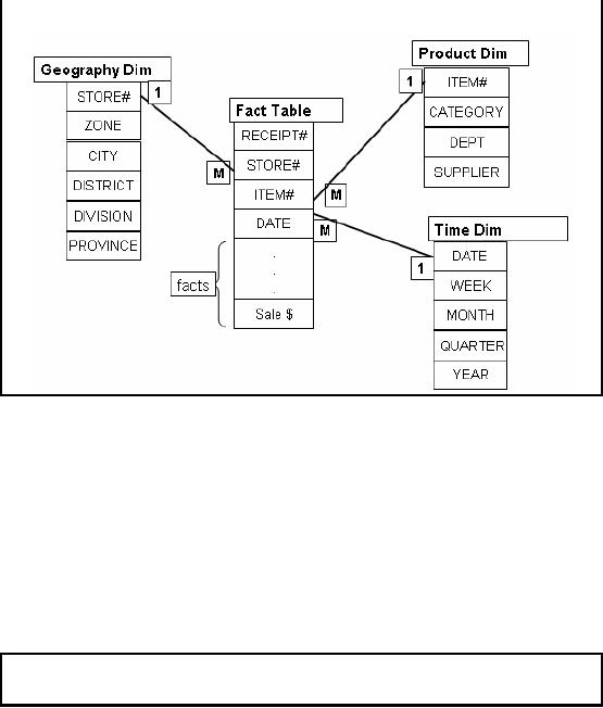
Figure-13.2: Dimensions have Hierarchies

The foundation for design in this environment is through use of dimensional modeling techniques

which focus on the concepts of "facts" and "dimensions" for organizing data.

Facts are the quantities or numerical measures (e.g., sales $) that we can count and the most

useful being those that are additive. The most useful facts in a fact table are numeric and additive.

Additive nature of facts is important, because data warehouse applications almost never retrieve a

single record form the fact table; instead, they fetch back hundreds, thousands, or even millions of

these records at a time, and the only useful thing to do with so many records is to add them up.

Example, what is the average salary of customers who's age > 35 and experience more than

5 years?

Dimensions are the descriptive textual information and the source of interesting constraints on

how we filter/report on the quantities (e.g., by geography, product, date, etc.). For the DM

shown, we constrain on the clothing department via the Dept attribute in the Product table. It

should be obvious that the power of the database shown is proportional to the quality and depth of

the dimension tables.

The two Schemas

Star

Snow-flake

Figure-13.3: The two schemas

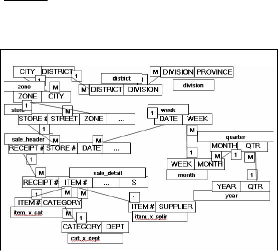
Fig-13.3 shows the snow-flake schema i.e. with multiple hierarchies that is typical of an OLTP or

MIS system. The other is a simplified star schema with no hierarchies and a central node. Such

schemas are typical of Data Warehouses.

Snowflake Schema: Sometimes a pure star schema might suffer performance problems. This can

occur when a de-normalized dimension table becomes very large and penalizes the star join

operation. Conversely, sometimes a small outer-level dimension table does not incur a significant

join cost because it can be permanently stored in a memory buffer. Furthermore, because a star

structure exists at the center of a snowflake, an efficient star join can be used to satisfy part of a

query. Finally, some queries will not access data from outer-level dimension tables. These queries

effectively execute against a star schema that contains smaller dimension tables. There fore, under

some circumstances, a snowflake schema is more efficient than a star schema.

Star Schema: A star schema is generally considered to be the most efficient design for two

reasons. First, a design with de-normalized tables encounters fewer join operations. Second, most

optimizers are smart enough to recognize a star schema and generate access plans that use

efficient "star join" operations. It has been established that a "standard template" data warehouse

query directly maps to a star schema.

"Simplified" 3NF (Retail)

Figure-13.4: "Simplified" 3NF (Retail)

In Fig -13.4 a (simplified) retail data model is shown in the third normal form representation keeps

each level of a dimensional hierarchy in a separate table (e.g., store, zone, region or item,

category, department). The sale header and detail information is also maintained in two separate

tables.

Vastly Simplified Star Schema

Figure-13.5: Vastly Simplified Star Schema

The goal of a star schema design is to simplify the physical data model so that RDBMS

optimizers can exploit advanced indexing and join techniques in a straightforward manner, as

shown in Fig-13.5. Some RDBMS products rely on star schemas for performance more than

others (e.g., Re d Brick versus Teradata).

The ultimate goal of a star schema design is to put into place a physical data model capable of

very high performance to support iterative analysis adhering to an OLAP model of data delivery.

Moreover, SQL generation is vastly simplified for front-end tools when the data is highly

structured in this way.

In some cases, facts will also be summarized along common dimensions of analysis for additional

performance.

The Benefit of Simplicity

Beauty lies in close correspondence with the business, evident even to business users.

The ultimate goal of a star schema design is to put into place a physical data model capable of

very high performance to support iterative analysis adhering to an OLAP model of data delivery.

Moreover, SQL generation is vastly simplified for front-end tools when the data is highly

structured in this way.

In some cases, facts will also be summarized along common dimensions of analysis for additional

performance.

Features of Star Schema

Dimens ional hierarchies are collapsed into a single table for each dimension. Loss of

information?

A single fact table created with a single header from the detail records, resulting in:

A vastly simplified physical data model!

Fewer tables (thousands of tab les in some ERP systems).

Fewer joins resulting in high performance.

Some requirement of additional space.

By "flattening" the information for each dimension into a single table and combining

header/detail records, the physical data model is vastly simplified. The simplified data model of a

star schema allows for straightforward SQL generation and makes it easier for RDBMS

optimizers detect opportunities for "star joins" as a means of efficient query execution.

Notice that star schema design is merely a specific methodology for deploying the pre-join de-

normalization that we discussed earlier.

Quantifying space requirement

Quantifying use of additional space using star schema

There are about 10 million mobile phone users in Pakistan.

Say the top company has half of them = 500,000

Number of days in 1 year = 365

Number of calls recorded each day = 250,000 (assumed)

Maximum number of records in fact table = 91 billion rows

Assuming a relatively small header size = 128 bytes

Fact table storage used = 11 Tera bytes

Average length of city name = 8 characters ≈ 8 bytes

Total number of cities with telephone access = 170 (1 byte)

Space used for city name in fact table using Star = 8 x 0.091 = 0.728 TB

Space used for city code using snow-flake = 1x 0.091= 0.091 TB

Additional space used ≈ 0.637 Tera byte i.e. about 5.8%

By virtue of flattening the dimensions, instead of storing the city code, now in the "flattened"

table the name of the city will be stored. There is a 1: 8 ratio between the two-representations. But

out of a header size of 128, there has been an addition of 7 more bytes i.e. an increase in storage

space of about 5%. This is not much, if there are frequent queries for which the join has not been

eliminated.

Table of Contents: