Describing Risk:Unequal Probability Outcomes

<< The Aggregate Demand For Wheat:NETWORK EXTERNALITIES

PREFERENCES TOWARD RISK:Risk Premium, Indifference Curve >>

Microeconomics ECO402

Lesson 13

Introduction

Choice with certainty is reasonably straightforward.

How do we choose when certain variables such as income and prices are uncertain (i.e.

making choices with risk)?

Describing Risk

To measure risk we must know:

1) All of the possible outcomes.

2) The likelihood that each outcome will occur (its probability).

Interpreting Probability

The likelihood that a given outcome will occur

Objective Interpretation

· Based on the observed frequency of past events

Subjective

· Based on perception or experience with or without an observed frequency

Different information or different abilities to process the same information can

influence the subjective probability

Expected Value

The weighted average of the payoffs or values resulting from all possible outcomes.

· The probabilities of each outcome are used as weights

· Expected value measures the central tendency; the payoff or value expected on

average

An Example

· Investment in drilling exploration:

· Two outcomes are possible

Success -- the stock price increase from $30 to $40/share

Failure -- the stock price falls from $30 to $20/share

· Objective Probability

100 explorations, 25 successes and 75 failures

Probability (Pr) of success = 1/4 and the probability of failure = 3/4

EV = Pr(success)($40/share) + Pr(failure)($20/share)

1 4 ($ 4 0 /s h a re ) + 3 4 ($ 2 0 /s h a re )

E V = $ 2 5 /s h a re

Given:

Two possible outcomes having payoffs X1 and X2

Probabilities of each outcome is given by Pr1 & Pr2

Generally, expected value is written as:

E(X) = Pr1X1 + Pr2X2 +... + Prn Xn

Microeconomics ECO402

Variability

The extent to which possible outcomes of an uncertain event may differ

Variability: A Scenario

Suppose you are choosing between two part-time sales jobs that have the same

expected income ($1,500)

The first job is based entirely on commission.

The second is a salaried position.

There are two equally likely outcomes in the first job--$2,000 for a good sales job and

$1,000 for a modestly successful one.

The second pays $1,510 most of the time (.99 probability), but you will earn $510 if the

company goes out of business (.01 probability).

Income from Sales Jobs

Outcome 1

Outcome 2

Probability

Income($)

probability

Income($)

Expected

income

2000

1000

1500

Job 1: Commission

.99

1510

.01

510

1500

Job 2: Fixed salary

E(X1 ) = .5($2000) + .5($1000) = $1500

Job 2 Expected Income

E(X 2 ) = .99($1510) + .01($510) = $1500

While the expected values are the same, the variability is not.

Greater variability from expected values signals greater risk.

Deviation

Difference between expected payoff and actual payoff

Deviations from Expected Income ($)

Outcome 1

Deviation

Outcome 2

Deviation

Job 1

$2,000

$500

$1,000

-$500

Job 2

1,510

510

-900

Adjusting for negative numbers

The standard deviation measures the square root of the average of the squares of the

deviations of the payoffs associated with each outcome from their expected value.

The standard deviation is written:

σ = Pr[X1 -E(X)2] +Pr [X2 -E(X)2]

Microeconomics ECO402

Calculating Variance ($)

Deviation

Standard

Outcome 1

Squared

Outcome 2

Squared Squared

Deviation

Job 1 $2,000

$250,000

$1,000

$250,000

$500.00

Job 2 1,510

100

510

980,100

9,900

99.50

The standard deviations of the two jobs are:

σ1 =

0) + .5($250,00

.5($250,00

σ 1 = $ 250 , 000

σ 1 = 500 *Greater Risk

+ .01($980,1

.99($100

00)

$ 9 , 900

= 99 . 50

The standard deviation can be used when there are many outcomes instead of only two.

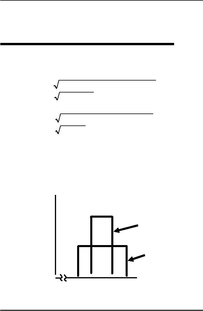
An Example

Job 1 is a job in which the income ranges from $1000 to $2000 in increments of $100

that are all equally likely.

Job 2 is a job in which the income ranges from $1300 to $1700 in increments of $100

that, also, are all equally likely.

Probability

Job 1 has greater

spread: greater

standard deviation

and greater risk

than Job 2.

0.2

Job 2

0.1

Job 1

Income

$1000

$1500

$2000

Outcome Probabilities of Two Jobs (unequal probability of outcomes)

Job 1: greater spread & standard deviation

Microeconomics ECO402

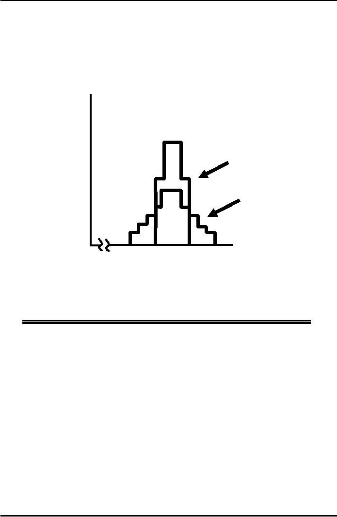
Peaked distribution: extreme payoffs are less likely

Decision Making

A risk avoider would choose Job 2: same expected income as Job 1 with less risk.

Suppose we add $100 to each payoff in Job 1 which makes the expected payoff =

$1600.

Unequal Probability Outcomes

The distribution of payoffs

Probability

associated with Job 1 has a

greater spread and standard

deviation than those with Job 2.

0.2

Job 2

0.1

Job 1

Income

$1000

$1500

$2000

Income from Sales Jobs--Modified ($)

Deviation

Deviation Standard

Outcome 1

Squared

Outcome 2

Squared

Squared Deviation

Job 1 $2,100

$250,000

$1,100

$250,000

$1, 600

$500

Job 2 1510

100

510

980,100

1, 500

99.50

Recall: The standard deviation is the square root of the deviation squared.

Decision making

Job 1: expected income $1,600 and a standard deviation of $500.

Job 2: expected income of $1,500 and a standard deviation of $99.50

Which job?

· Greater value or less risk?

Example

Suppose a city wants to deter people from wrong parking.

The alternatives ......

Microeconomics ECO402

Assumptions:

1) Wrong parking saves a person $5 in terms of time spent searching for a parking space.

2) The driver is risk neutral.

3) Cost of apprehension is zero.

A fine of $5.01 would deter the driver from double parking.

Benefit of wrong parking ($5) is less than the cost ($5.01) equals a net benefit that is

less than 0.

Increasing the fine can reduce enforcement cost:

A $50 fine with a .1 probability of being caught results in an expected penalty of $5.

A $500 fine with a .01 probability of being caught results in an expected penalty of $5.

The more risk averse drivers are, the lower the fine needs to be in order to be effective.

Table of Contents: