DeNormalization Techniques: Splitting Tables, Horizontal splitting, Vertical Splitting, Pre-Joining Tables, Adding Redundant Columns, Derived Attributes

<< De-Normalization: Balance between Normalization and De-Normalization

Issues of De-Normalization: Storage, Performance, Maintenance, Ease-of-use >>

Lecture Handout

Data Warehousing

Lecture No. 08

De-Normalization Techniques

Splitting Tables

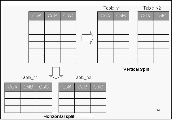
Figure-8.1: Splitting Tables

Splitting Tables

The denormalization techniques discussed earlier all dealt with combining tables to avoid doing

run-time joins by decreasing the number of tables. In contrast, denormalization can be used to

create more tables by splitting a relation into multiple tables. Both horizontal and vertical splitting

and their combination are possible. This form of denormalization -record splitting - is especially

common for a distributed DSS environment.

Splitting Tables: Horizontal splitting

Breaks a table into multiple tables based upon common column values. Example: Campus

spec ific queries.

GOAL

Spreading rows for exploiting parallelism.

Grouping data to avoid unnecessary query load in WHERE clause.

Splitting Tables

Horizontal splitting breaks a relation into multiple record set specifications by placing different

rows into different tables based upon common column values. For the multi-campus example

being considered; students from Islamabad campus in the Islamabad table, Peshawar students in

corresponding table etc. Each file or table created from the splitting has the same record lay out or

header.

Goals of Horizontal splitting:

There are typically two specific goals for horizontal partitioning: (1) spread rows in a large table

across many HW components (disks, controllers, CPUs, etc.) in the environment to facilitate

parallel processing, and (2) segregate data into separate partitions so that queries do not need to

examine all data in a table when WHERE clause filters specify only a subset of the partitions. Of

course, what we would like in an ideal deployment is to get both of these benefits from table

partitioning.

Advantages of Splitting tables:

Horizontal splitting makes sense when different categories of rows of a table are processed

separately: e.g. for the student table if a high percentage of queries are focused towards a certain

campus at a time then the table is split accordingly. Horizontal splitting can also be more secure

since file level of security can be used to prohibit users from seeing certain rows of data. Also

each split table can be organized differently, appropriate for how it is individually used. In terms

of page access, horizontally portioned files are likely to be retrieved faster as compared to un -split

files, because the latter will involve more blocks to be accessed.

Splitting Tables: Horizontal splitting

ADVANTAGE

Enhance security of data.

Organizing tables differently for different queries.

Reduced I/O overhead.

Graceful degradation of database in case of table damage.

Fewer rows result in flatter B-trees and fast data retrieval.

Other than performance, there are some other very useful results of horizontal splitting the tables.

As we discussed in the OLAP lecture, security is one of the key features required from an OLAP

system. Actually DSS is a multi-user environment, and robust security needs to ensure. By

splitting the tables and restricting the users to a particular split actually improves the security of

the system. Consider time -based queries, if the queries have to cover last years worth of data,

then splitting the tables on the basis of year will defiantly improve the performance as the amount

of data to be accessed is reduced. Similarly, if for a multi-campus university, most of the queries

are campus specific, then splitting the tables based on the campus wou ld result in improved

performance. In both of the cases of splitting discussed i.e. time and space, as the number of

records to be retrieved is reduced, resulting in more records per block that translates into fewer

page faults and high performance. If the table is not partitioned, and for some reason the table is

damaged, then in the worst case all data might be lost. However, when the table gets partitioned,

and even if a partition is damaged, ALL of the data is not lost. Assuming a worst case scenario

that tables crash i.e. all of them, the system will not go down suddenly, but would go down

gradually i.e. gracefully.

Splitting Tables: Vertical Splitting

Splitting and distributing into separate files with repeating primary key.

Infrequently accessed columns become extra "baggage" thus degrading performance.

Very useful for rarely accessed large text columns with large headers.

Header size is reduced, allowing more rows per block, thus reducing I/O.

For an end user, the split appears as a single table through a view.

Splitting Tables: Vertical Splitting

Vertical splitting involves splitting a table by columns so that a group of columns is placed into

the new table and the remaining columns are placed in another new table. Thus columns are

distributed into separate files, such that the primary key is repeated in each of the files. An

example of vertical splitting would be breaking apart the student registration table by creating a

personal_info table by placing SID along with corresponding data into one record specification,

the SID along with demographic-related student data into another record specification, and so on.

Vertical splitting can be used when some columns are rarely accessed rather than other columns

or when the table has wide rows or header or both. Thus the infrequently accessed columns

become extra "baggage" degrading performance. The net result of splitting a table is that it may

reduce the number of pages/blocks that need to be read because of the shorter header length

allowing more rows to be packed in a block, thus reducing I/O. A vertically split table should

contain one row per primary key in the split tables as this facilitates data retrieval across tables

and also helps in dissolving the split i.e. making it reversible. In reality, the users are unaware of

the split, as view of a joined table is presented to the users.

2. Pre-Joining

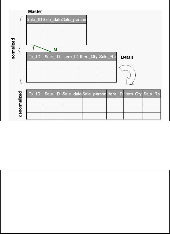
Pre-Joining

Figure-8.2: Pre-joining Tables

The objective behind pre-joining is to identify frequent joins and append the corresponding tables

together in the physical data model. This technique is generally used when there is a one-to-

many relationship between two (or more) tables, such as the master-detail case when there are

header and detail tables in the logical data model. Typically, referential integrity is assumed from

the foreign key in one table (detail) to the primary key in the other table (header).

Additional space will be required, because information on the master table is stored once for each

detail record i.e. multiple times instead of just once as would be the case in a normalized design.

Pre-Joining

Typical of Market basket query

Join ALWAYS required

Tables could be millions of rows

Squeeze Master into Detail

Repetition of facts. How much?

Detail 3-4 times of master

Figure -8.2 shows a typical case of market basket querying, with a master table and a detail table.

The sale_ID column is the primary key for the master table and uniquely identifies a market

basket. There will be on e "detail" record for each item listed on the "receipt" for the market

basket. The tx_ID column is the primary key for the detail table.

Observe that in a normalized design the store and sale date for the market basket is on one table

(master) and the item (along with quantity, sales Rs, etc.) are on a separate table (detail). Almost

all analysis will require product, sales date, and (sometimes) sale person (in the context of HR).

Moreover, both tables can easily be millions of rows for a large retail outlet with significant

historical data. This means that a join will be forced between two very large tables for almost

every query asked of the data warehouse. This could easily choke the system and degrade

performance.

Note that this same header/detail structure in the data applies across many industries as we have

discussed in the very early lectures, such as healthcare, transportation, logistics, billing etc.

To avoid the run-time join, we use the pre-join technique and "squeeze" the sales master

information into the detail table. The obvious drawback is repetition of facts from the master

table into the detail table. This avoids the join operation at run -time, but stores the header

information redundantly as part of the sales detail. This redund ant storage is a violation of

normalization, but will be acceptable if the cost of storage is less then the performance achieved

by virtue of eliminating the join.

4. Adding Redundant Columns

This technique can be used when a column from one table is frequently accessed in a large scale

join in conjunction with a column from another table. To avoid this join, the column is added

(redundant) or moved into the detail table(s) to avoid the join. For example, if frequent joins are

performed using Table_1 and Table_2 using columns ColA, ColB and ColC, then it is suitable to

add ColC to Table_1.

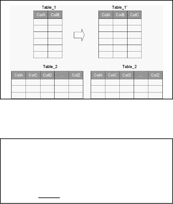
Adding Redundant Columns

Figure-8.3: Adding redundant columns

Note that the columns can also be moved, instead of making them redundant. If closely observed,

this technique is no different from a pre -joining. In pre-joining all columns are moved from the

master table into the detail table, but in the current case, a sub-set of columns from the master

table is made redundant or moved into the detail table. The performance, and storage trade-offs

are also very similar to pre -joining.

Adding Redundant Columns

Columns can also be moved, instead of making them redundant. Very similar to pre -joining as

discussed earlier.

EXAMPLE

Frequent referencing of code in one table and corresponding description in another table.

A join required is required.

To eliminate the join, a redundant attribute added in the target entity which is

functionally independent of the primary key.

A typical scenario for column redundancy/movement is frequent referencing of code in one table

and the corresponding description in another table. The description of a code is retrieved via a

join. In such a case, redundancy will naturally pay off. This is implemented by duplicating the

descriptive attribute in the entity, which would otherwise contain only the code. The result is a

redundant attribute in the target entity which is functionally independent of the primary key. Note

that this foreign key relationship was created in the first place to normalize the corresponding

description reduce update anomalies.

Redundant Columns: Surprise

Note that:

§ Actually increases in storage space, and increase in update overhead.

Keeping the actual table intactand unchanged helps enforce RI constraint.

Age old debate of RI ON or OFF.

Redundant Columns Surprise

Creating redundant columns does not necessarily reduce the storage space requirements, as

neither the reference table is removed, nor the columns duplicated from the reference table.

The reason being to ensure data input RI constraint, although this reasoning falls right in the

middle of the age old debate that Referential Integrity (RI) constraint should be turned ON or

OFF in a DWH environment. However, it is obvious that column redundancy does eliminate the

join and increase the performance.

Derived Attributes

Objectives

§ Ease of use for decision support applications

§ Fast response to predefined user queries

§ Customized data for particular target audiences

§ Ad-hoc query support

Feasible when...

§ Calculated once, used most

§ Remains fairly "constant"

§ Looking for absoluteness of correctness.

Pitfall of additional space and query degradation.

5. Derived Attributes

It is usually feasible to add derived attribute(s) in the data warehouse data model, if the derived

data is frequently accessed and calculated once and is fairly stable. The justification of adding

derived data is simple; it reduces the amount of query processing time at run -time while accessi g

the data in the warehouse. Furthermore, once the data is properly calculated, there is little or no

apprehension about the authenticity of the calculation. Put in other words, once the derived data is

properly calculated it kind of becomes absolute i.e. there is hardly any chance that someone might

use a wrong formula to calculate it incorrectly. This actually enhances the credibility of the data

in the data warehouse.

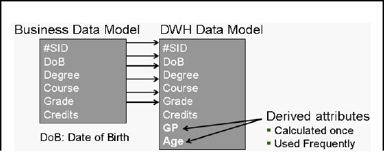
Derived Attributes

Figure-8.4: Business Data Model vs. DWH Data Model

GP (Grade Point) column in the data warehouse data model is included as a derived value. The

formula for calculating this field is Grade*Credits.

Age is also a derived attribute, calculated as Current_Date DoB (calculated periodically).

In most cases, it will only make sense to use derived data if the ratio of detail rows to derived

rows is at least 10:1. In such cases, the 10% storage cost for keeping the derived data is less than

the temporary and sort space storage costs for many concurrent queries aggregating at runtime.

Table of Contents: