Cost in the Long Run:Long-Run Cost with Economies & Diseconomies of Scale

<< A Firm’s Short-Run Costs ($):The Effect of Effluent Fees on Firms’ Input Choices

Production with Two Outputs--Economies of Scope:Cubic Cost Function >>

Microeconomics ECO402

Lesson 20

Cost in the Long Run

Cost minimization with Varying Output Levels

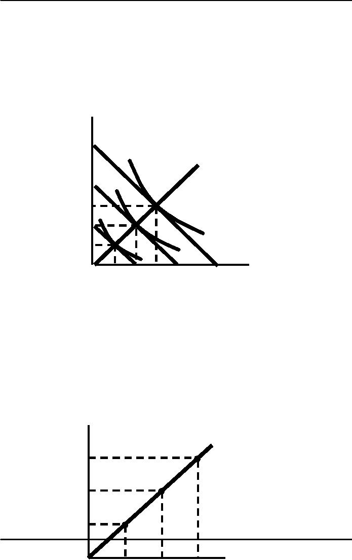
A firm's expansion path shows the minimum cost combinations of labor and capital at each

level of output.

A Firm's

The expansion path illustrates

Capital

the least-cost combinations of

per

labor and capital that can be

year

used to produce each level of

output in the long-run.

150 $3000 Isocost Line

Expansion Path

$2000

Isocost Line

100

300 Unit Isoquant

200 Unit

Isoquan

Labor per year

100

150

200

300

Expansion Path

Cost

per

Year

Expansion Path

3000

A firm's Long

2000

run total

cost curve

1000

100

Output, Units/yr

100

200

300

Microeconomics ECO402

Long-Run Versus Short-Run Cost Curves

What happens to average costs when both inputs are variable (long run) versus only having

one input that is variable (short run)?

101

Microeconomics ECO402

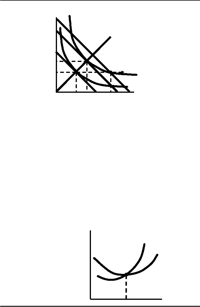
The Inflexibility of Short-Run Production

Capital

The long-run expansion

per

path is drawn as before..

year

Long-Run

Expansion Path

Short-Run

Expansion Path

L3 D

Labor per year

Long-Run Average Cost (LAC)

Constant Returns to Scale

·If input is doubled, output will double and average cost is constant at all levels of output.

Increasing Returns to Scale

·If input is doubled, output will more than double and average cost decreases at all levels

of output.

Decreasing Returns to Scale

·If input is doubled, the increase in output is less than twice as large and average cost

increases with output.

In the long-run:

·Firms experience increasing and decreasing returns to scale and therefore long-run

average cost is "U" shaped.

Long-run marginal cost leads long-run average cost:

·If LMC < LAC, LAC will fall

·If LMC > LAC, LAC will rise

·Therefore, LMC = LAC at the minimum of LAC

Long-Run Average and Marginal Cost

Cost($

per unit

output

Output

102

Microeconomics ECO402

Question

What is the relationship between long-run average cost and long-run marginal cost when

long-run average cost is constant?

Economies and Diseconomies of Scale

Economies of Scale

·Increase in output is greater than the increase in inputs.

Diseconomies of Scale

·Increase in output is less than the increase in inputs.

Measuring Economies of Scale

Ec = Cost - output elasticity

= %Δ in cost from a 1% increase

in output

Therefore, the following is true:

EC< 1: MC < AC

·Average cost indicate decreasing economies of scale

EC = 1: MC = AC

·Average cost indicate constant economies of scale

EC > 1: MC > AC

·Average cost indicate increasing economies of scale

The Relationship Between Short-Run and Long-Run Cost

We will use short and long-run cost to determine the optimal plant size

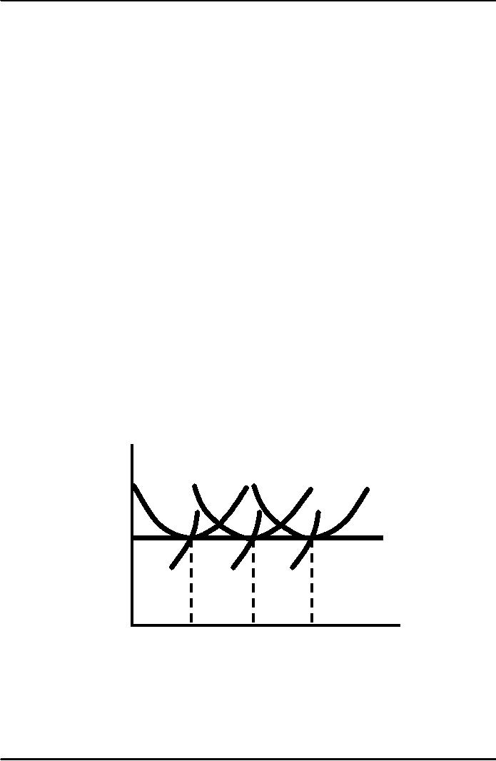
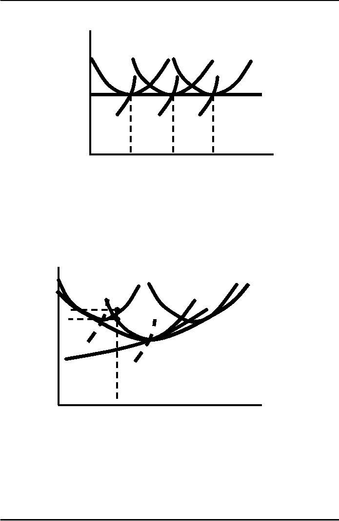
Long-Run Cost with Constant Returns to Scale

Cost

With many plant sizes with SAC = $10

($ per unit

the LAC = LMC and is a straight line

of output

SAC1

SAC2

SAC3

SMC2

SMC3

SMC

LAC =

LMC

Output

Observation

The optimal plant size will depend on the anticipated output (e.g. Q1 choose SAC1,etc).

The long-run average cost curve is the envelope of the firm's short-run average cost curves.

Question

What would happen to average cost if an output level other than that shown is chosen?

103

Microeconomics ECO402

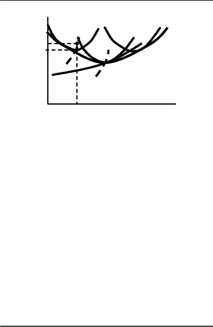
Long-Run Cost with Economies & Diseconomies of Scale

Cost

SAC1

($ per unit

LAC

SAC3

of output

SAC2

$10

If the output is Q1 a

SMC1

SMC3

manager

would chose the small

LMC

SMC2

plant

SAC1 and SAC $8.

Output

What is the firms' long-run cost curve?

Firms can change scale to change output in the long-run.

The long-run cost curve is the dark blue portion of the SAC curve which represents the

minimum cost for any level of output.

Observations

The LAC does not include the minimum points of small and large size plants? Why not?

LMC is not the envelope of the short-run marginal cost. Why not?

Measuring Economies of Scale

Ec = (ΔC/ C) /(ΔQ/ Q)

Ec =(ΔC/ ΔQ)/(C/ Q) = M /A

C C

Therefore, the following is true:

EC< 1: MC < AC

· Average cost indicate decreasing economies of scale

EC = 1: MC = AC

· Average cost indicate constant economies of scale

EC > 1: MC > AC

· Average cost indicate increasing economies of scale

The Relationship Between Short-Run and Long-Run Cost

We will use short and long-run cost to determine the optimal plant size

104

Microeconomics ECO402

Long-Run Cost with Constant Returns to Scale

Cost

With many plant sizes with SAC = $10

($ per unit

the LAC = LMC and is a straight line

of output

SAC1

SAC2

SAC3

SMC2

SMC3

SMC

LAC =

LMC

Output

Observation

The optimal plant size will depend on the anticipated output (e.g. Q1 choose SAC1,etc).

The long-run average cost curve is the envelope of the firm's short-run average cost

curves.

Question

What would happen to average cost if an output level other than that shown is chosen?

Long-Run Cost with Economies & Diseconomies of Scale

Cost

SAC1

($ per unit

LAC

SAC3

of output

SAC2

$10

If the output is Q1 a

manager

SMC1

SMC3

would chose the small

plant

LMC

SAC1 and SAC $8.

SMC2

Output

What is the firms' long-run cost curve?

Firms can change scale to change output in the long-run.

The long-run cost curve is the dark blue portion of the SAC curve which represents the

minimum cost for any level of output.

Observations

The LAC does not include the minimum points of small and large size plants? Why not?

LMC is not the envelope of the short-run marginal cost. Why not?

105

Table of Contents: