 |
Case Study: Agri-Data Warehouse |
| << Contents of Project Reports |
| Web Warehousing: Drawbacks of traditional web sear ches, web search, Web traffic record: Log files >> |
Lecture-38
Case
Study: Agri-Data
Warehouse
Step 6:
Data Acquisition &
Cleansing
Trained
scouts from DPWQCP
periodically visit randomly selected
points and manually note
35
attributes,
with some given in Table 2.
These hand-written sheets
are subsequently filed. For
the
last 10
years, the data collected
was recorded by typing the
hand -filled pest scouting
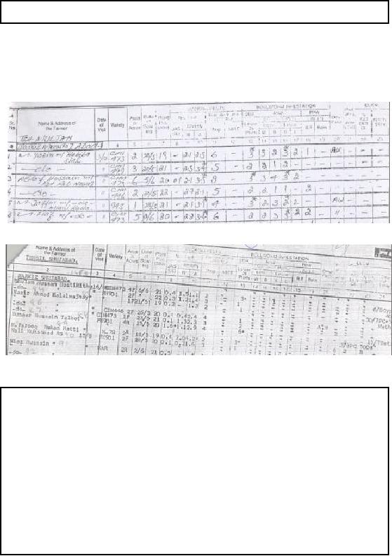
sheets. Copy
of a hand
filled pest scouting sheet
is shown in Figure -38.1(a).
Figure-38.1(a):
Hand filled Pest Scouting
sheet
Figure-38.1(b):
Typed Pest Scouting
sheet
The * in Figure
-38.1 corresponds to pest hot spot or
flare-up or ETL_A.
Step-6:
Issues
�
The
pest scouting sheets are
larger than A4 size (8.5" x
11"), hence the right
end was
cropped when
scanned on a flat -bed A4 size
scanner.
�
The
right part of the scouting
sheet is also the most
troublesome, because of
pesticide
names
for a single record typed on
multiple lines i.e. for
multiple farmers.
�
As a first
step, OCR (Optical Character
Reader) based image to text
transformation of the
pest
scouting sheets was
attempted. But it did not
work even for relatively
clean sheets
with
very high scanning
resolutions.
�
Subsequently
DEO's (Data Entry Operators) were employed to
digitize the scouting
sheets by
typing.
318

The
pest scouting sheets are
larger than A4 size (8.5" x
11"), hence the right
end was cropped
when
scanned on a flat -bed A4
size scanner. The right
part of the scouting sheet is
also the most
troublesome,
because of pesticide names
for a single record typed on
multiple lines i.e.
for
multiple
farmers.
As a first
step, OCR (Optical Character
Reader) based image to text
transformation of the pest
scouting sheets
was attempted. But it did not
work even for relatively
clean sheets with very
high
scanning
resolutions, such as 600 dpi.
Subsequently DEO's (Data Entry Operators)
were
employed to
digitize the scouting sheets
by typing. To reduce spelling errors in pesticide
names
and
addresses, drop down menu or
combo boxes with standard
and correct names were
created
and
used.
Step-6:
Why the issues?
�
Major
issues of data cleansing had
arisen due to data
processing and handling at
four
levels by
different groups of
people
1. Hand
recordings by the scouts at
the field level.
2. Typing
hand recordings into data
sheets at the DPWQCP
office.
3. Photocopying
of the typed sheets by
DPWQCP personnel.
4. Data entry or
digitization by hired data entry
operators.
Data
cleansing and standardization is probably
the largest part in an ETL
exercise. For Agri -
DWH
major issues of data
cleansing had arisen due to
data processing and handling
at four levels
by different
groups of people i.e. (i)
Hand recordings by the scouts at
the field level (ii)
typin g
hand recordings
into data sheets at the
DPWQCP office (iii) photocopying of the
scouting sheets
by DPWQCP
personnel and finally (iv)
data entry or digitization by hired
data entry operators.
After
achieving acceptable level of
data quality, the data was
loaded into Teradata
data
warehouse;
subsequently each column was probed
using SQL for erroneous
entries. Some of the
errors
found were correct data in
wrong columns, nonstandard or
invalid variety names etc.
There
were some
intrinsic errors, such as variety type
"999" or spray_date "12:00:00 AM"
inserted by
the
system against missing
values. Variations found in pesticide
names and cotton variety
names
were removed by
comparing them with standard
names.
Step 7:
Data Transform, Transport &
Populate
Among
the different types of
transformations performed in the
implementation, only the
more
complex
i.e. multiple M:1
transformations for field
individualization will be discussed in
this
section.
Motivation
for Transformation
�
Trivial
queries give wrong
results.
�
Static
and dynamic
attributes
�
Static
attributes recorded
repeatedly.
Table 2
gives details of the main
attributes recorded at each point.
Static attributes are
those
attributes
that are recorded on each
visit by the scouts, usually
does not changes.
319
Static
Attributes
Dynamic
Attributes
1
Farmer
Name
1
Date of
Visit
2
Farmer
Address
2
Pest
Population
3
Field
Acreage
3
CLCV
4
Variety(ies)
Sown
4
Predator
Population
5
Sowing
date
5
Pesticide
Spray Dates
6
Sowing
method
6
Pesticide(s)
Used
Table-38.1:
Cotton pest scouting attributes
recorded by DPWQCP
surveyors
The
data recorded consists of
two parts i.e. static
and dynamic (Table -38.1). On
each visit, the
static, as
well as the dynamic data is
recorded by the scouts, thus
resulting in stat ic values
getting
recorded
repeatedly. Since no mechanism is
used to uniquely identify
each and every
farmer,
therefore,
trivial queries, such as total
area scouted, distribution of varieties
sown etc. gives
wrong
results. For example, while
aggregating area, the area
of the farmer with multiple
visits
during
the season is counted
multiple times, giving incorrect
results, same is true for
varieties
sown.
Therefore, to do any reasonable
analysis after data
cleansing, the most important
step of
data
transformation being individualization of the
cultivated fields, not farmers. The
reason being,
a farmer
usually has multiple fields,
but a field is associated or owned by a
single farmer.
Step-7:
Resolving the
issue
�
Solution:
Individualization
of cultivated fields.
� Technique similar to
BSN used to fix
names.
� Unique ID
assigned to farmers.
� BSN used
again, and unique ID assigned to
fields.
�
Results:
�
Limitation:
Field
individualization not perfect.
Some cases of farmers with
same
geography,
sowing date, same variety
and same area. Such
cases were dropped.
Method
Field
individualization turned out to be a very laborious
process. It was attempted by
first
uniquely
identifying the farmers.
This was achieved by collectivity sorting
farmer name, Mozua
and
Markaz. The
grouping of farmer names was
scrutinized to fix the spelling
errors in the farmer
names
and unique farmer_ID was
assigned to each farmer. Subsequently
based on the
farmer_ID,
sowing date,
area and variety, cultivated
fields were uniquely
identified and field_ID
assigned to
each
field.
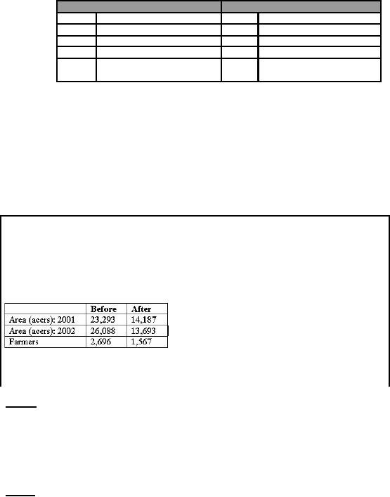
Results
To demonstrate
the amount of error removed
because of field individualization,
consider the case
of scouted
area and unique farmers. Without
field individualization, the
cotton scouted area
for
2001
and 2002 added to 23,293
and
26,088
acres,
respectively. After field
individualization, the
correct
scouted area turned out to be 14,187 and
13,693
acres
respectively i.e. a correction of
about
50%. Similarly unique farmers
reduced from 2,696
to
1,567. The
method of field
320

individualization
is in no way perfect, there were some
cases of farmers with same
geography,
sowing date,
same variety and same
area. Such cases were
dropped.
Transporting the
data
Once
the data entry was complete,
double checked and reconciled
the corresponding files
were
compressed
and moved from the
premises of the DEO (Data Entry Operator)
to the University,
where sample
printout of data entered were
taken and a final random
quality check was
performed.
Subsequently minor errors, if
any were fixed and data
was loaded into the
Agri-DWH.
Step 8:
Determine Middleware
Connectivity
Since
the source data is
maintained in a non digital format,
hence connectivity with the
data
warehouse
was irrelevant. Once digitized, it
was rather trivial to load the
data into the
warehouse.
Furthermore, in
the foreseeable future, it
was not anticipated that the
scouting sheets were
going
to be maintained
in a digitized form.
Steps
9-11: Prototyping, Querying &
Reporting
�
Implemented the
prototype with user
involvement.
�
Applications
developed
� 10.
A
data mining tool was
also developed based on an indigenous
technique that
used
crossing minimization paradigm for
unsupervised clustering.
�
11. A low-cost OLAP
tool was indigenously developed; actually
it was a Multi
dimensional
OLAP or MOLAP.
�
Use querying
& reporting tools
�
The
following SQL query was
used for validation:
SELECT
Date_of_Visit, AVG(Predators),
..............................................................AVG(Dose1+Dose2+Dose3+Dose4)
FROM
Scouting_Data
WHERE
Date_of_Visit < #12/31/2001# and
predators > 0
GROUP BY
Date_of_Visit;
Implement a
prototype with user
involvement
The
Agri-DWH was implemented
with the involvement of the
end users. In this regard
there was
close
collaboration between the development
team and personnel of (i)
Directorate of Pest
Warning, Multan
(ii) National Agriculture
Research Center (NARC),
Islamabad (iii)
Pakistan
Agriculture
Research Council (PARC) and
(iv) Agriculture University,
Faisalabad. The
implementation
was centered around numerous
meetings with the potential
end users, discussion
of results,
and also explicit set of
questions provided by
them.
Applications
developed
A low-cost
OLAP tool was indigenously developed;
actually it was a Multi
dimensional OLAP or
MOLAP. Using
the MOLAP tool, agriculture extension
data was analyzed. A data
mining tool
was
also developed based on an indigenous
technique that used crossing
minimization paradigm
for
unsupervised clustering.
Use querying
& reporting tools
321

Despite
small number of rows i.e.
4,400, the Agri-DWH was
implemented using Teradata
for the
sake of
completion of the entire cycle. The
following SQL query was used
to generate Figure -
38.2.
SELECT
Date_of_Visit, AVG(Predators),
AVG(Dose1+Dose2+Dose3+Dose4)
FROM
Scouting_Data
WHERE
Date_of_Visit < #12/31/2001# and
predators > 0
GROUP BY
Date_of_Visit;
Step
12: Deployment & System
Management
Since
Agri-DWH was a pilot
project, therefore, the traditional
deployment methodologies
and
system
management techniques were not
followed to the word, and
are not discussed
here.
Decision
Support using
Agri-DWH
Agri-DSS
usage: Data
Validation
�
Quality and
validity of the underlying
data is the key to
meaningful and
authentic
analysis.
�
After
ensuring a satisfactory level of
data quality (based on
cost-benefit trade-off)
extremely
important to scientifically validate the
data that the DWH
will constitute.
�
Some
very natural checks were
employed for this purpose.
Relationship between
the
pesticide
spraying and predator (beneficial insects)
population is a fact well
understood
by
agriculturists.
�
Predator
population decreases as pesticide spray
increases and then continually
decreases
till
the end of season.
Quality
and validity of the
underlying data is the key
to meaningful and authentic
analysis. After
ensuring a
satisfactory level of data
quality (based on cost-benefit trade-off)
it is extremely
important to
somehow judge the validity of
data that a data warehouse
constitutes. Some
very
natural
checks were employed for
this purpose. Relationship
between the pesticide
spraying and
predator
(beneficial insects) population is a fact
well understood by agriculturists.
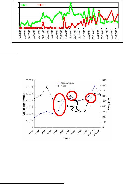
Predator
population
decreases as pesticide spray
increases and then
continually decreases till
the end of
season, as
shown in Fig-38.2. In Figure -38.2 the y
-axis shows the relative
frequency of pesticide
sprays in
multiple of 100 ml, and average
predators population greater than
zero.
322
10
Predator
Spray
8
6
4
2
0
Figure
38.2: Year 2001 Frequency of spray Vs.
Predators population
FAO
Report
Pesticides
are used as means for
increasing production, as a positive correlation is
believed to
exist
between yield and pesticide
usage. However, existence of an
undesirable, sometime
even
negative correlation
between pesticide usage and
yield has been observed in
Pakistan (FAO: Food
and
Agriculture Organization report 2001).
Figure-38.3 shows a marked
decrease in yield
while
the
pesticide usage is on the
rise, and also its
converse, creating a complex
situation.
Negative
correlation
Figure
38.3: Yield and Pestici de
Usage in Pakistan: Source
FAO (2001)
Excessive
use of pesticides is harmful in
multiple ways. On one hand,
farmers have to pay more
for
the pesticides, while on the
other, increased pesticide
usage develops immunity in pests,
thus
making them more
harmful to the crops.
Excessive usage of many
pesticides is also harmful
for
the
environment and hazardous to
human.
Reasons
for pesticide abuse can be
discovered by automatically exploring pest
scouting and
metrological
data.
Working
Behaviors at Field Level: Spray
dates
As expected,
the results of querying for
spray dates and spray
frequency for 2001 and 2002 do
not
display
any well defined patterns; as it is
dependent on pest populations
(Fig -37.2), availability of
pesticides
etc. To study the relationsh
ip between sprays and time,
moving average of sprays
for
five
days, and a moving correlation of
sprays for five days were
calculated. For the sake
of
323
uniformity,
the moving average of spray
was normalized using the maximum
spray frequency.
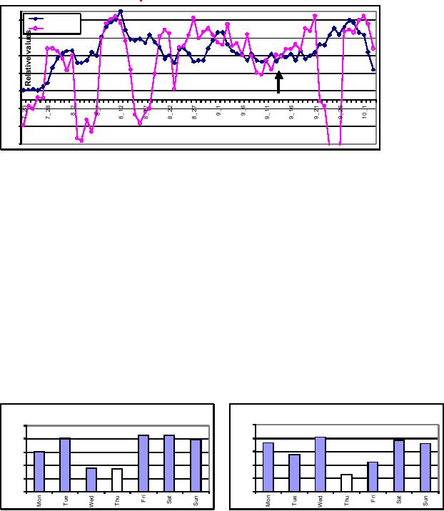
The
results are shown in Figure
-38.4.
Moving
Avg
0.90
Correlation
0.70
0.50
0.30
0.10
-0.10
-0.30
Spray
dates (mm_dd) for 2001 &
2002
-0.50
Figure-38.4(a):
Spray frequency Vs. day of
year for Year
2001
No relationship
should have existed for
the two years. But note
the surprising finding that
most
sprays
occurring on and around 12th Aug. in BOTH years
with high co rrelation, appearing as
a
spike.
Also note the dip in
sprays around 11th
Sep.! Sowing at
predetermined time makes
sense,
as it is under
the control of the farmer, but
that is not true for
spraying. Pests don't
follow
calendars;
therefore, whenever, ETL_A is crossed
pesticides are
sprayed.
14th Aug. is the independence
day of Pakistan and a national holiday.
In Pakistan, people are in
a
habit of sandwiching
gazetted holidays with
casual leaves; consequently
businesses are closed
for
a longer period,
including that of pesticide
suppliers. 14th
Aug.
occurred on Tue and Wed in
2001
and
2002, respectively, thus making it ideal
to stretch the weekend.
During Aug/Sep. humidity
is
also high,
with correspondingly high chances of
pest infestations. Therefore,
appare ntly the
farmers decided
not to take any chances, and
started spraying around 11th Aug.;
evidently even
when it
was not required. Unfortunately, the
weather forecast for 13 Aug.
2001 and 2002 was
showers
and cloudy, respectively.
Therefore, most likely the
pesticide sprayed was washed
-off.
Unfortunately
the decline in sprays around
9/11 could not be
explained.
Working
Behaviors at Field Level: Sowing
dates
The
results of querying the sowing date
based on the day of the
week are shown in
Fig-38.5.
2002:
Sowing week_day
2001:
Sowing week_day
500
500
431
429
409
405
398
387
367
357
400
400
303
278
300
300
223
179
174
200
200
124
100
100
0
0
Figure
38.5: Number of sowings against week
days
324
Observe least
number of sowings done on Thursdays, in
each year. This finding
was later
confirmed by
extension personnel. Multan is
famous for its shrines.
Thursdays are usually
related
with religious
festi vals and activities, a mix of
devotion and recreation, and
usually held at
shrines,
hence a tendency of doing
less work on Thursdays.
Similar behavior was
observed for
spraying
too.
Conclusions
& lessons learnt
� Extract
Transform Load (ETL) of agricultural
extension data is a big
issue. There are no
digitized
operational databases so one has to
resort to data available in
typed (or hand
written)
pest
scouting sheets. Data entry of
these sheets is very
expensive, slow and prone to
errors.
� Particular to
the pest scouting data,
each farmer is repeatedly
visited by agriculture extension
people.
This results in repetition of
information, about land, sowing
date, variety etc
(Table-2).
Hence,
farmer and land individualization
are critical, so that repetition may
not impair
aggregate
queries. Such an individualization
task is hard to implement for
multiple reasons.
� There is a
skewness in the scouting
data. Public extension personnel
(scouts) are more likely
to
visit
educated or progressive farmers, as it
makes their job of data
collection easy. Furthermore,
large land
owners and influential farmers
are also more frequently
visited by the scouts.
Thus
the
data does not give a true
statistical picture of the farmer
demographics.
� Unlike
traditional data warehouse where the
end users are decision
makers, here the decision
-
making goes
all the way "down" to
the extension level. This
presents a challenge to
the
analytical operations'
designer, as the findings
must be fairly simple to
understand and
communicate.
325
Table of Contents:
- Need of Data Warehousing
- Why a DWH, Warehousing
- The Basic Concept of Data Warehousing
- Classical SDLC and DWH SDLC, CLDS, Online Transaction Processing
- Types of Data Warehouses: Financial, Telecommunication, Insurance, Human Resource
- Normalization: Anomalies, 1NF, 2NF, INSERT, UPDATE, DELETE
- De-Normalization: Balance between Normalization and De-Normalization
- DeNormalization Techniques: Splitting Tables, Horizontal splitting, Vertical Splitting, Pre-Joining Tables, Adding Redundant Columns, Derived Attributes
- Issues of De-Normalization: Storage, Performance, Maintenance, Ease-of-use
- Online Analytical Processing OLAP: DWH and OLAP, OLTP
- OLAP Implementations: MOLAP, ROLAP, HOLAP, DOLAP
- ROLAP: Relational Database, ROLAP cube, Issues
- Dimensional Modeling DM: ER modeling, The Paradox, ER vs. DM,
- Process of Dimensional Modeling: Four Step: Choose Business Process, Grain, Facts, Dimensions
- Issues of Dimensional Modeling: Additive vs Non-Additive facts, Classification of Aggregation Functions
- Extract Transform Load ETL: ETL Cycle, Processing, Data Extraction, Data Transformation
- Issues of ETL: Diversity in source systems and platforms
- Issues of ETL: legacy data, Web scrapping, data quality, ETL vs ELT
- ETL Detail: Data Cleansing: data scrubbing, Dirty Data, Lexical Errors, Irregularities, Integrity Constraint Violation, Duplication
- Data Duplication Elimination and BSN Method: Record linkage, Merge, purge, Entity reconciliation, List washing and data cleansing
- Introduction to Data Quality Management: Intrinsic, Realistic, Orr’s Laws of Data Quality, TQM
- DQM: Quantifying Data Quality: Free-of-error, Completeness, Consistency, Ratios
- Total DQM: TDQM in a DWH, Data Quality Management Process
- Need for Speed: Parallelism: Scalability, Terminology, Parallelization OLTP Vs DSS
- Need for Speed: Hardware Techniques: Data Parallelism Concept
- Conventional Indexing Techniques: Concept, Goals, Dense Index, Sparse Index
- Special Indexing Techniques: Inverted, Bit map, Cluster, Join indexes
- Join Techniques: Nested loop, Sort Merge, Hash based join
- Data mining (DM): Knowledge Discovery in Databases KDD
- Data Mining: CLASSIFICATION, ESTIMATION, PREDICTION, CLUSTERING,
- Data Structures, types of Data Mining, Min-Max Distance, One-way, K-Means Clustering
- DWH Lifecycle: Data-Driven, Goal-Driven, User-Driven Methodologies
- DWH Implementation: Goal Driven Approach
- DWH Implementation: Goal Driven Approach
- DWH Life Cycle: Pitfalls, Mistakes, Tips
- Course Project
- Contents of Project Reports
- Case Study: Agri-Data Warehouse
- Web Warehousing: Drawbacks of traditional web sear ches, web search, Web traffic record: Log files
- Web Warehousing: Issues, Time-contiguous Log Entries, Transient Cookies, SSL, session ID Ping-pong, Persistent Cookies
- Data Transfer Service (DTS)
- Lab Data Set: Multi -Campus University
- Extracting Data Using Wizard
- Data Profiling