Bundling:Mixed Versus Pure Bundling, Effects of Advertising

<< Bundling:Consumption Decisions When Products are Bundled

MONOPOLISTIC COMPETITION:Monopolistic Competition in the Market for Colas and Coffee >>

Microeconomics ECO402

Lesson 38

Bundling

Mixed Bundling

Selling both as a bundle and separately

Pure Bundling

Selling only a package

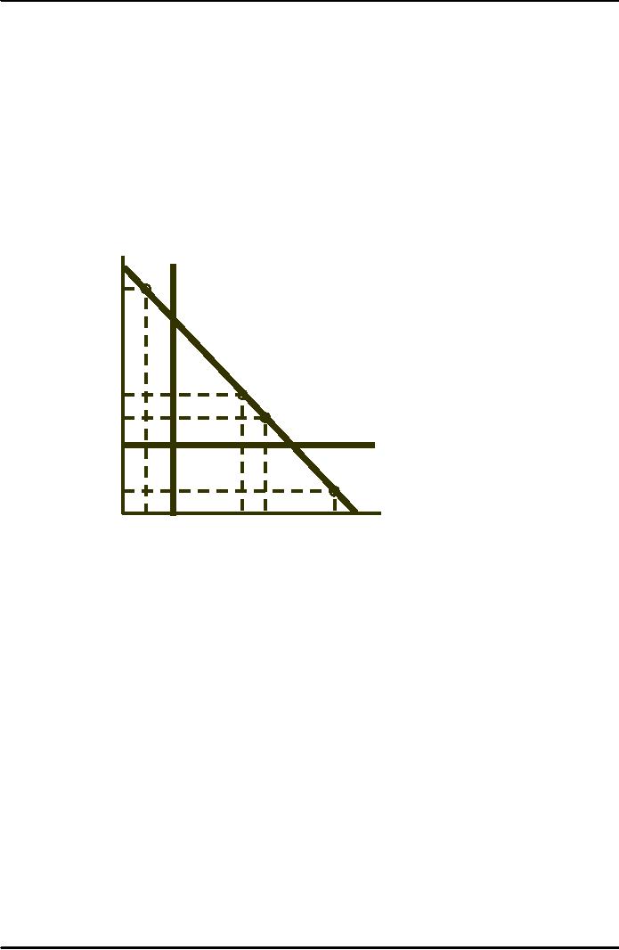
Mixed Versus Pure Bundling

C1 = MC1

C1 = 20

With positive marginal

costs, mixed bundling

100

may be more profitable

than pure bundling.

Consumer A, for example, has

a reservation price for good 1

that is below marginal cost c1.

With mixed bundling, consumer A

is induced to buy only good 2, while

consumer D is induced to buy only good 1,

reducing the firm's cost.

C2 = MC2

C2 = 30

10 20 30 40 50 60 70 80 90 100

Mixed vs. Pure Bundling

Scenario

Perfect negative correlation

Significant marginal cost

Observations

Reservation price is below MC for some consumers

Mixed bundling induces the consumers to buy only goods for which their reservation

price is greater than MC

Bundling Example

Sell Separately

Consumers B,C, and D buy 1 and A buys 2

Pure Bundling

Consumers A, B, C, and D buy the bundle

Mixed Bundling

Consumer D buys 1, A buys 2, and B & C buys the bundle

174

Microeconomics ECO402

Profit

Sell separately

$50

$90

----

$150

Pure bundling

----

$100

$200

Mixed bundling

$89.95

$89.95 $100

$229.90

C1 = $20

C2 = $30

Sell Separately

3($50 - $20) + 1($90 - $30) = $150

Pure Bundling

4($100 - $20 - $30) = $200

Mixed Bundling

($89.95 - $20) + ($89.95 - $30) - 2($100 - $20 - $30) = $229.90

C1 = $20 C2 = $30

Question

If MC = 0, would mixed bundling still be the most profitable strategy with perfect negative

correlation?

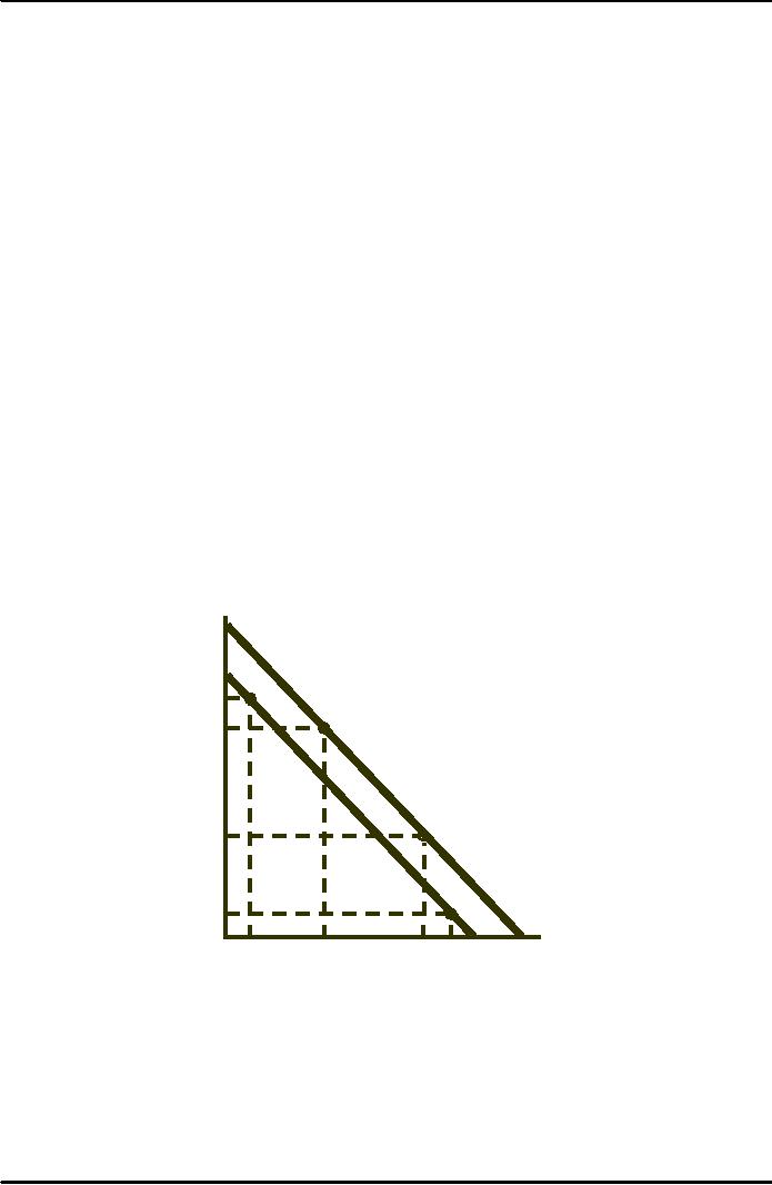
Mixed Bundling with Zero Marginal Costs

r2 120

In this example, consumers B and C

are willing to pay $20 more for the bundle

than are consumers A and D. With

100

mixed bundling, the price of the bundle

can be increased to $120. A & D can be

charged $90 for a single good.

80 9

100

120

Profit

Sell separately

$80

----

$320

Pure bundling

----

$100

$400

Mixed bundling

$90

$120

$420

175

Microeconomics ECO402

Bundling in Practice

Automobile option packages

Vacation travel

Cable television

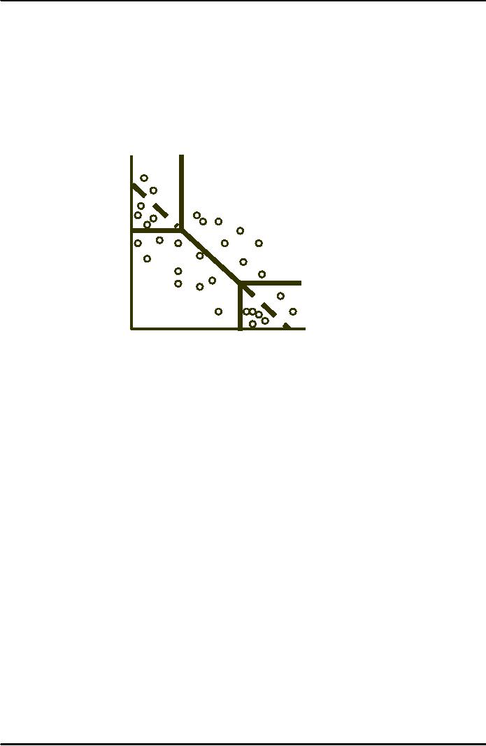
Mixed Bundling in Practice

Use of market surveys to determine reservation prices

Design a pricing strategy from the survey results

The dots are estimates of

reservation prices for a

representative sample of

consumers.

The firm can first choose a price

for the bundle and then try individual

prices P1 and P2 until total profit

is roughly maximized.

The Complete Dinner vs. a la Carte:

A Restaurant's Pricing Problem

Pricing to match consumer preferences for various selections

Mixed bundling allows the customer to get maximum utility from a given expenditure by

allowing a greater number of choices.

Bundling

Tying

Practice of requiring a customer to purchase one good in order to purchase another.

Examples

Xerox machines and the paper

IBM mainframe and computer cards

Allows the seller to meter the customer and use a two-part tariff to discriminate against

the heavy user

McDonald's

Allows them to protect their brand name.

Advertising

Assumptions

Firm sets only one price

Firm knows Q(P,A)

How quantity demanded depends on price and advertising

176

Microeconomics ECO402

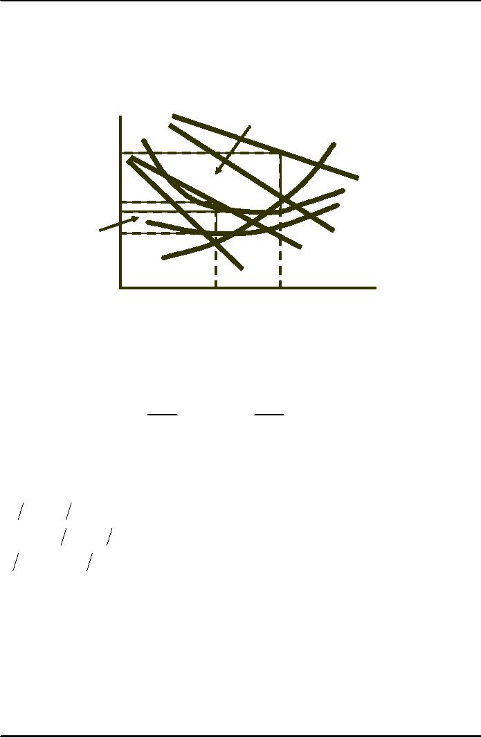
Effects of Advertising

AR and MR are

If the firm advertises, its average

average and marginal

and marginal revenue curves shift

revenue when the firm

to the right -- average costs

doesn't advertise.

rise, but marginal cost

does not.

š1

$/Q

AR'

AC'

š0

MR'

Quantity

Advertising

š = PQ ( P , A ) - C ( Q ) - A

ΔQ

MR Ads = P

= 1 + MC

= full MC of adv.

ΔA

Choosing Price and Advertising Expenditure

A Rule of Thumb for Advertising

( A Q)(ΔQ ΔA) = EA = Adv. elasticity of demand

(P - MC ) P = -1 EP

A PQ = -(EA EP ) = Rule of Thumb

To maximize profit, the firm's advertising-to-sales ratio should be equal to minus the

ratio of the advertising and price elasticities of demand.

R(Q) = $1 million/yr

$10,000 budget for A (advertising--1% of revenues)

EA = .2 (increase budget $20,000, sales increase by 20%

EP = -4 (markup price over MC is substantial)

Question

Should the firm increase advertising?

177

Microeconomics ECO402

YES

A/PQ = -(2/-.4) = 5%

Increase budget to $50,000

Questions

When EA is large, do you advertise more or less?

When EP is large, do you advertise more or less?

Advertising: In Practice

Estimate the level of advertising for each of the firms

Supermarkets

EP= -10; EA = 0.1 to 0.3

Convenience stores

EP= -5; EA = very small

Designer jeans

EP= -3 to -4; EA= 0.3 to 1

Laundry detergents

EP= -3 to -4; EA= very large

178

Table of Contents: