 |
Monopsony Power:Pricing With Market Power, Capturing Consumer Surplus |
| << The Social Costs of Monopoly Power:Price Regulation, Monopsony |
| Monopsony Power:THE ECONOMICS OF COUPONS AND REBATES >> |

Microeconomics
ECO402
VU
Lesson
34
Monopsony
Power
A
few
buyers can influence price
(e.g. automobile industry).
Monopsony
power gives them the
ability to pay a price that
is less than marginal
value.
The
degree of monopsony power
depends on three similar
factors.
1)
Elasticity of market
supply
�The less elastic
the market supply, the
greater the monopsony
power.
2)
Number of buyers
�The fewer the
number of buyers, the less
elastic the supply and
the greater the
monopsony
power.
3)
Interaction Among
Buyers
�The less the
buyers compete, the greater
the monopsony power.
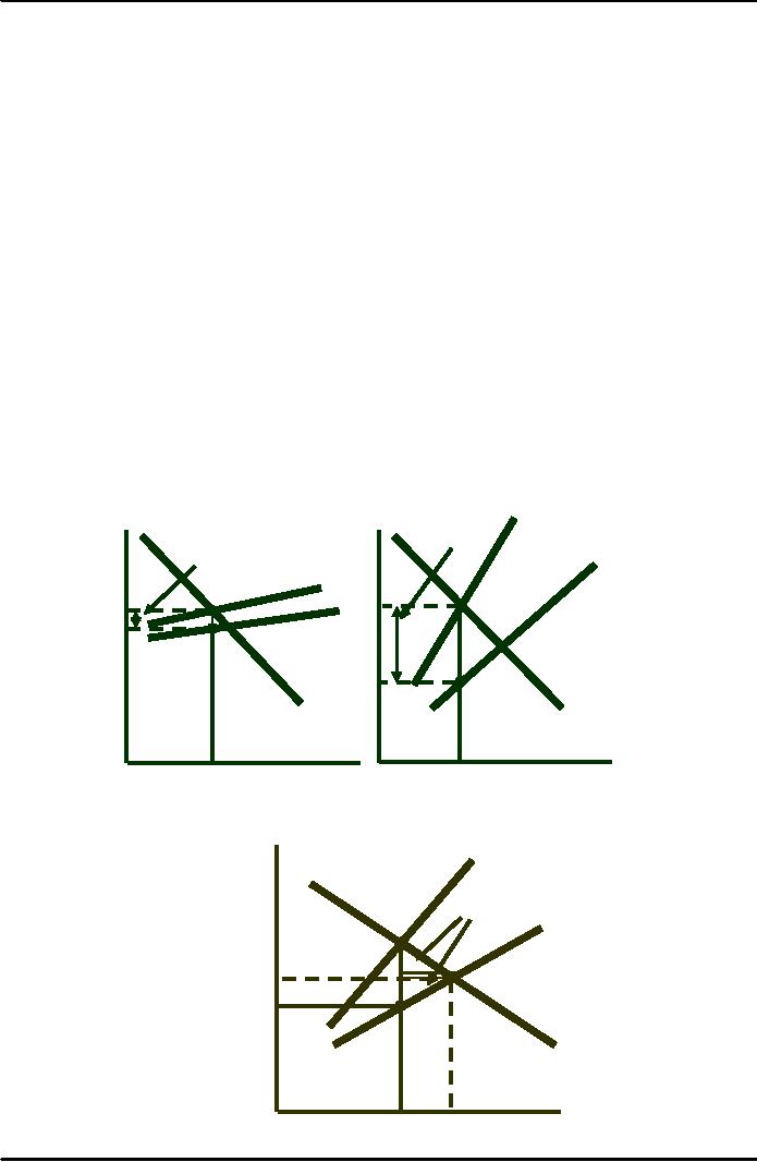
Monopsony
Power:
If
the Elastic versus Inelastic
Supply
ME
MV
- P*
$/Q
$/Q
MV
- P*
S
= AE
ME
S
= AE
P*
P*
MV
MV
Quantity
Q*
Q*
Quantity
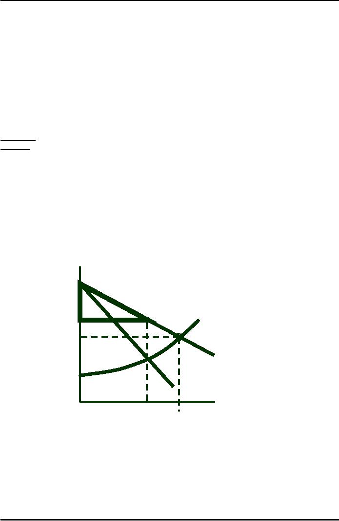
Deadweight
Loss from Monopsony Power in
the
$/Q
ME
Deadweight
Loss
S
= AE
B
PC A
C
P*
MV
Q*
QC
Quantity
158

Microeconomics
ECO402
VU
Determining
the deadweight loss in
monopsony
Change in
seller's surplus =
-A-C
Change in
buyer's surplus = A - B
Change in
welfare = -A - C + A - B = -C - B
Inefficiency
occurs because less is
purchased
The
Social Cost of Monopsony
Power
Bilateral
Monopoly
�
Bilateral
monopoly
is
rare, however, markets with
a small number of sellers
with
monopoly
power selling to a market
with few buyers with
monopsony power is
more
common.
Question
�
In this
case, what is likely to
happen to price?
Limiting
Market Power: The Antitrust
Laws
Antitrust
Laws:
Promote a
competitive economy
Rules and
regulations designed to promote a
competitive economy
by:
�
Prohibiting
actions that restrain or are
likely to restrain
competition
�
Restricting
the forms of market
structures that are
allowable
Pricing
With Market Power
Pricing
without market power
(perfect competition) is determined by
market supply and
demand.
The
individual producer must be
able to forecast the market
and then concentrate
on
managing
production (cost) to maximize
profits.
Pricing
with market power (imperfect
competition) requires the
individual producer to
know
much
more about the
characteristics of demand as well as
manage production.
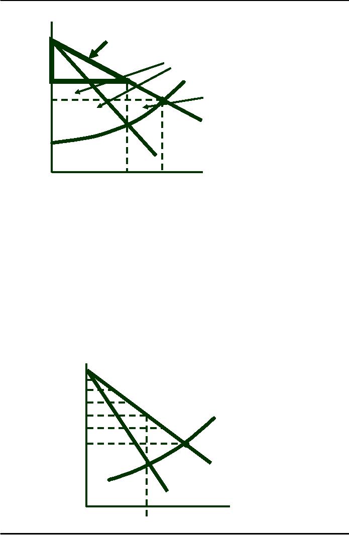
Capturing
Consumer Surplus
Between
0 and Q*,
consumers
$/Q
Pma
A
will
pay more than
P*--consumer
surplus (A).
P1
PC is
the price
that
would exist in
B
P*
a
perfectly
competitive
P2
If
price is raised above
M
P*,
the firm will
lose
PC
sales
and reduce profit.
D
Beyond
Q*, price will
have
to fall to create a
consumer
surplus (B).
M
Quantity
Q*
159

Microeconomics
ECO402
VU
Capturing
Consumer Surplus
�P*Q*:
single
P &
Q @
MC=MR
�A:
consumer
surplus with P*
�B:
P>MC & consumer
would buy
at
a lower price
�P1:
less
sales and profits
�P2 :
increase
sales & and reduce
revenue
and profits
�PC: competitive
price
Question
How can the firm
capture the consumer surplus
in A
and
sell profitably in B?
Answer
Price discrimination Two-part
tariffs Bundling
Price
discrimination is the charging of
different prices to different
consumers for similar
goods.
Price
Discrimination
First
Degree Price
Discrimination
Charge a
separate price to each
customer: the maximum or
reservation
price they
are
willing
to pay.
Additional
Profit From Perfect
First-Degree Price
Discrimination
Without
price discrimination,
output
is Q* and price is
P*.
$/Q
Variable
profit is the area
Pmax
Consumer
surplus is the area
between
the MC & MR.
above
P* and between
0
and Q* output.
MC
P*
With
perfect discrimination,
each
consumer
pays the maximum
price
they are willing to
pay.
PC
D
= AR
Output
expands to Q** and
price
falls
to PC where
MC = MR = AR
=
D.Profits increase by the
area
MR
above
MC
between
old MR and D to
output
Q**
Quantity
Q*
Q**
160

Microeconomics
ECO402
VU
With
perfect discrimination
�
Each
customer pays their
Consumer
surplus when a
$/Q
Pmax
reservation
price
single
price P* is charged.
�Profits increase
Variable
profit when a
single
price P* is charged.
MC
P*
Additional
profit from
perfect
price discrimination
PC
D
= AR
MR
Quantity
Q*
Q**
Question
Why would a
producer have difficulty in
achieving first-degree price
discrimination?
Answer
1)
Too many customers
(impractical)
2)
Could not estimate the
reservation price for each
customer
First
Degree Price
Discrimination
The model
does demonstrate the
potential profit (incentive) of
practicing price
discrimination
to some degree.
Examples of
imperfect price discrimination
where the seller has
the ability to
segregate
the
market to some extent and
charge different prices for
the same product:
Lawyers,
doctors, accountants
Car
salesperson (15% profit
margin)
Colleges
and universities
First-Degree
Price Discrimination in
Practice
Six
prices exist
resulting
$/Q
in
higher profits. With a
single price
P1
P*4,
there are few consumers
and
those
who pay P5 or
P6 may have a
P2
surplus.
P3
MC
P*4
P5
P6
D
MR
Quantity
Q
161

Microeconomics
ECO402
VU
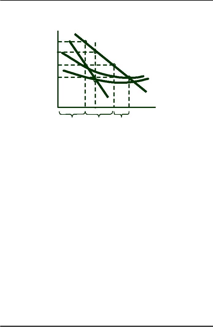
Second-Degree
Price Discrimination
Second-degree
price
discrimination
is pricing
$/Q
according
to quantity
consumed--or
in blocks.
P1
Without
discrimination: P = P0
and
Q = Q0.
With second-
P0
degree
discrimination
there are three
prices
P1,
P2, and P3.
(e.g.
electric utilities)
P2
AC
P3
MC
D
MR
Q0
Q1
Q2
Q3
Quantity
1st
2nd
3rd
Economies
of scale permit:
�Increase consumer
welfare
�Higher profits
162
Table of Contents:
- ECONOMICS:Themes of Microeconomics, Theories and Models
- Economics: Another Perspective, Factors of Production
- REAL VERSUS NOMINAL PRICES:SUPPLY AND DEMAND, The Demand Curve
- Changes in Market Equilibrium:Market for College Education
- Elasticities of supply and demand:The Demand for Gasoline
- Consumer Behavior:Consumer Preferences, Indifference curves
- CONSUMER PREFERENCES:Budget Constraints, Consumer Choice
- Note it is repeated:Consumer Preferences, Revealed Preferences
- MARGINAL UTILITY AND CONSUMER CHOICE:COST-OF-LIVING INDEXES
- Review of Consumer Equilibrium:INDIVIDUAL DEMAND, An Inferior Good
- Income & Substitution Effects:Determining the Market Demand Curve
- The Aggregate Demand For Wheat:NETWORK EXTERNALITIES
- Describing Risk:Unequal Probability Outcomes
- PREFERENCES TOWARD RISK:Risk Premium, Indifference Curve
- PREFERENCES TOWARD RISK:Reducing Risk, The Demand for Risky Assets
- The Technology of Production:Production Function for Food
- Production with Two Variable Inputs:Returns to Scale
- Measuring Cost: Which Costs Matter?:Cost in the Short Run
- A Firm’s Short-Run Costs ($):The Effect of Effluent Fees on Firms’ Input Choices
- Cost in the Long Run:Long-Run Cost with Economies & Diseconomies of Scale
- Production with Two Outputs--Economies of Scope:Cubic Cost Function
- Perfectly Competitive Markets:Choosing Output in Short Run
- A Competitive Firm Incurring Losses:Industry Supply in Short Run
- Elasticity of Market Supply:Producer Surplus for a Market
- Elasticity of Market Supply:Long-Run Competitive Equilibrium
- Elasticity of Market Supply:The Industry’s Long-Run Supply Curve
- Elasticity of Market Supply:Welfare loss if price is held below market-clearing level
- Price Supports:Supply Restrictions, Import Quotas and Tariffs
- The Sugar Quota:The Impact of a Tax or Subsidy, Subsidy
- Perfect Competition:Total, Marginal, and Average Revenue
- Perfect Competition:Effect of Excise Tax on Monopolist
- Monopoly:Elasticity of Demand and Price Markup, Sources of Monopoly Power
- The Social Costs of Monopoly Power:Price Regulation, Monopsony
- Monopsony Power:Pricing With Market Power, Capturing Consumer Surplus
- Monopsony Power:THE ECONOMICS OF COUPONS AND REBATES
- Airline Fares:Elasticities of Demand for Air Travel, The Two-Part Tariff
- Bundling:Consumption Decisions When Products are Bundled
- Bundling:Mixed Versus Pure Bundling, Effects of Advertising
- MONOPOLISTIC COMPETITION:Monopolistic Competition in the Market for Colas and Coffee
- OLIGOPOLY:Duopoly Example, Price Competition
- Competition Versus Collusion:The Prisoners’ Dilemma, Implications of the Prisoners
- COMPETITIVE FACTOR MARKETS:Marginal Revenue Product
- Competitive Factor Markets:The Demand for Jet Fuel
- Equilibrium in a Competitive Factor Market:Labor Market Equilibrium
- Factor Markets with Monopoly Power:Monopoly Power of Sellers of Labor