 |
Assignment Problems:SOLUTION OF AN ASSIGNMENT PROBLEM |
| << Assignment Problems:MATHEMATICAL FORMULATION OF THE PROBLEM |
| Queuing Theory:DEFINITION OF TERMS IN QUEUEING MODEL >> |
Operations
Research (MTH601)
203
Subject
to restrictions,
Row
restrictions
x11 +
x12 + x13
+ x14 =
1
for
job 1
x21 +
x22 + x23
+ x24 =
1
for
job 2
x31 +
x32 + x33
+ x34 =
1
for
job 3
x41 +
x42 + x43
+ x44 =
1
for
job 4
Column
restrictions
x11 +
x21 + x31
+ x41 =
1
for
person 1
x12 +
x22 + x32
+ x42 =
1
for
person 2
x13 +
x23 + x33
+ x43 =
1
for
person 3
x14 +
x24 + x34
+ x44 =
1
for
person 4
xij = 0 or
1
and
In
general,
xi1 +
xi2 + ... + xin
= 1, for i =
1, 2, ..., n
x1j +
x2j + ... + xnj
= 1, for j =
1, 2, ..., n
and
When
compared with a transportation
problem, we see that
ai = 1
and
bj = 1 for
all rows and columns,
xij = 0 or
1.
We
shall not attempt simplex
algorithem or the transportation
algorithm to get a
solution
to an assignment problem. Certain
systematic procedure has
been devised so as to
obtain
the solution to the problem with
ease.
SOLUTION
OF AN ASSIGNMENT PROBLEM
The
solution to an assignment problem is
based on the following
theorem.
Theorem:
If
in an assignment problem we add a
constant to every element of a
row or column in the
effectiveness
matrix then an assignment
that minimizes the total
effectiveness in one matrix
also minimizes the
total
effectiveness in the other
matrix.
Example:
A
works manager has to
allocate four different jobs to four workmen.
Depending on the
efficiency
and the capacity of the
individual the times taken
by each differ as shown in
the table 2. How
should
the
tasks be assigned one jot to
a worker so as to minimize the total
man-hours?
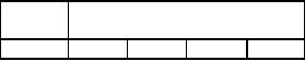
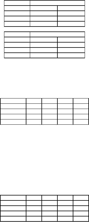
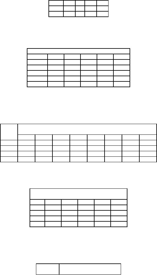
Table
2
Worker
Job
A
B
C
D
1
10
20
18
14
203
Operations
Research (MTH601)
204
2
15
25
9
25
3
30
19
17
12
4
19
24
20
10
The
following steps are followed
to find an optimal
solution.
Solution:
STEP
1:Consider
each row. Select the
minimum element in each row.
Subtract this smallest
element form all
the
elements in that row. This
results in the table
3.
Table
3
Worker
Job
A
B
C
D
1
0
10
8
4
2
6
16
0
16
3
18
7
5
0
4
9
14
10
0
STEP
2:
We subtract the minimum
element in each column from
all the elements in its column.
Thus we obtain
table
4
Table
4
Worker
Job
A
B
C
D
1
0
3
8
4
2
6
9
0
16
3
18
0
5
0
4
9
7
10
0
STEP
3:In
this way we make sure
that in the matrix each
row and each column has
atleast one zero
element.
Having
obtained atleast one zero in
each row and each column, we
assign starting from first
row.
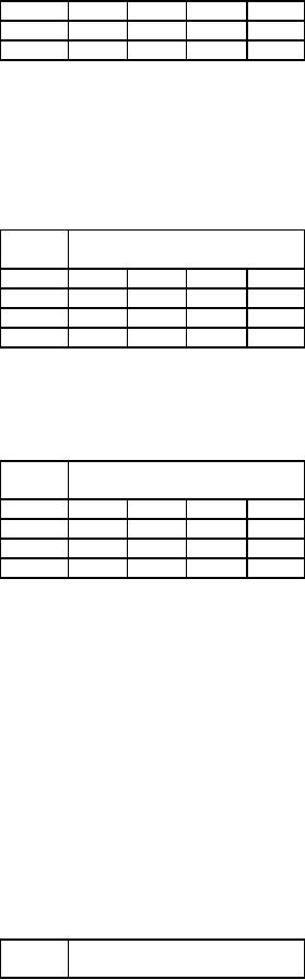
In
the first row, we have a
zero in (1, A). Hence we
assign job 1 to the worker
A. This assignment is
indicated
by
a square .
All
other zeros in the column
are crossed (X) to show
that the other jobs
cannot be assigned to
worker
A as he has already been
assigned. In the above
problem we do not have other
zeros in the first
column
A.
Proceed
to the second row. We have a
zero in (2, C). Hence we
assign the job 2 to worker
C, indicating by a
square
.
Any
other zero in this column is
crossed (X).
Proceed
to the third row. Here we
have two zeros corresponding
to (3, B) and (3, D).
Since there is a tie for
the
job
3, go to the next row deferring
the decision for the
present. Proceeding to the fourth
row, we have only
one
zero
in (4, D). Hence we assign
job 4 to worker D. Now the column D has a
zero in the third row. Hence
cross
(3,
D). All the assignments made
in this way are as shown in
table 5.
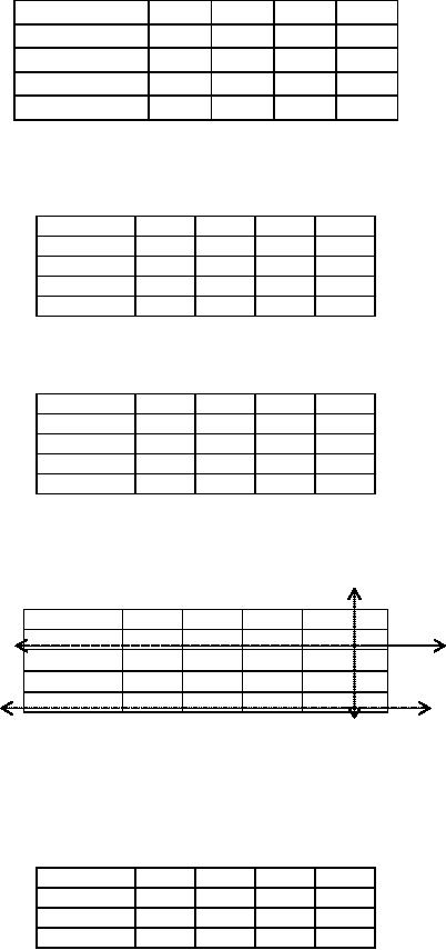
Table
5
Worker
Job
A
B
C
D
204
Operations
Research (MTH601)
205
1
0
3
8
4
2
6
9
0
14
3
18
0
5
0
4
9
7
10
0
STEP
4:
Now having assigned certain
jobs to certain workers we proceed to
the column 1. Since there is
an
assignment
in this column, we proceed to the second
column. There is only one
zero in the cell (3,
B); we assign
the
jobs 3 to worker B. Thus all
the four jobs have been
assigned to four workers. Thus we
obtain the solution to
the
problem as shown in the
table 6.
Table
6
Worker
Job
A
B
C
D
1
0
3
8
4
2
6
9
0
16
3
18
0
5
0
4
9
7
10
0
The
assignments are
Job
to Worker
1
A
2
C
3
B
4
D
We
summarise the above
procedure as a set of following
rules:
a.
Subtract
the minimum element in each
row from all the
elements in its row to make
sure that at least
we
get one zero in that
row.
b.
Subtract
the minimum element in each
column from all the elements
in its
column
in
the
above
reduced
matrix, to make sure that we
get at least one zero in
each column.
c.
Having
obtained at least one zero
in each row and atleast
one zero in each column,
examine rows
successively
until a row with exactly one
unmarked zero is found and
mark ( ) this
zero, indicating
that
assignment in made there.
Mark (X) all other
zeros in the same column, to show
that they cannot
be
used to make other
assignments. Proceed in this way
until all rows have been
examined. If there is a
tie
among zeros defer the
decision.
Next
consider columns, for single
unmarked zero, mark them ( ) and
d.
mark
(X) any other
unmarked
zero
in their rows.
e.
Repeat
(c) and (d) successively
until one of the two
occurs.
205
Operations
Research (MTH601)
206
1)
There are no zeros left
unmarked.
2)
The remaining unmarked zeros
lie atleast two in each
row and column. i.e., they
occupy
corners
of a square.
If
the outcome is (1), we have
a maximal assignment. In the
outcome (2) we use arbitrary
assignments. This
process
may yield multiple
solutions.
206
Operations
Research (MTH601)
207
MULTIPLE
SOLUTIONS
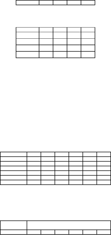
Example
1 Given
the following matrix, find
the optimal
assignment.
1
2
3
4
5
5
0
3
2
6
1
0
0
5
4
7
2
0
3
0
4
0
3
0
1
0
3
0
4
6
5
0
0
0
5
Solution:
Note
that all the rows and
columns have at least one
zero.
Row
1 has a single zero in column 2. So
make an assignment, delete (mark X)
the second zero in
0
denotes
assignment
column
2. This is shown in table 7.
Table
7
1
2
3
4
5
1
0
5
3
2
6
2
0
0
5
4
7
3
0x
3
0
4
0
4
0x
1
0
3
0
5
0
6
5
0x
0x
Row
2 has a single zero in the
first column. So make an assignment
and delete the remaining
zeros in column 1
as
shown in table 8.
Table
8
1
2
3
4
5
1
0
5
3
2
6
2
0
0x
5
4
7
3
0x
3
0
4
0
207
Operations
Research (MTH601)
208
4
0x
1
0
3
0
5
6
5
0
0
0
Row
3, 4 and 5 have more than a
single zero. So we skip these rows
and examine the columns.
Columns 3 has
three
zeros and so omit it. Column
4 has a single zero in row
5. So we make an assignment, deleting
the
remaining
zeros in row 5. The result
is as shown in table 9.
Table
9
1
2
3
4
5
1
0
5
3
2
6
2
0
0x
5
4
7
0x
3
0
4
0
3
0x
1
0
3
0
4
0
5
6
5
0x
0x
Now
we have two zeros in rows 3
and 4 in columns 3 and they
occupy the corners of a
square. An arbitrary
assignment
has to be made. If we make an
assignment in (3, 3) and
delete the remaining zero in
row 3 and in
column
3, this leaves one zero in
the position (4, 5) and an
assignment is made there.
Thus we have a solution to
the
problem as in table
10.
Table
10
1
2
3
4
5
1
0
3
2
6
5
0
0x
5
4
7
2
3
0
0x
3
4
0x
0
0
1
0x
3
4
0
5
0x
6
5
0
One
more assignment (as a solution) is
possible in this problem.
(i.e.) we could have made an
assignment at (3,
5)
deleting other zero in the
row 3 and zero in column 5
and making the last
assignment at (4, 3). This is
shown
below
in table 11.
208
Operations
Research (MTH601)
209
Table
11
1
2
3
4
5
1
0
3
2
6
5
2
0
0x
5
4
7
3
0
0x
3
0x
4
4
0
3
0x
0x
1
5
0
0x
6
5
0x
All
the above markings can be
done in a single matrix
itself. We need not write
the matrix
Remark:
repeatedly.
This is done only to clarify
the presentation.
HUNGARIAN
ALGORITHM
In
the two examples above,
the first one gave a
solution leaving no zeros. It was a
case of no ambiguity
and
in the second, we had more
zeros and the tie was
broken arbitrarily. Sometimes if we
proceed in the steps
explained
above, we get a maximal
assignment, which does not
contain an assignment in every
row or column.
We
are faced with a question of
how to solve the problem. In
such a case, the
effectiveness matrix has to
be
modified,
so that after a finite
number of iterations an optimal
assignment will be in sight.
The following is the
algorithm
to solve a problem of this
kind and this is known as
Hungarian algorithm. The systematic
procedure is
explained
in different steps and a problem is
solved as an illustration.
STEP
1:
Starting with a maximal
assignment mark (√
)
all rows for which
assignments have not been
made.
STEP
2:Mark
(√
)
columns not already marked
which have zeros in the
marked-rows.
STEP
3:Mark
(√
)
rows not already marked
which have assignments in
the marked columns.
STEP
4:Repeat
steps 2 and 3 until the
chain of markings
ends.
STEP5:
Draw lines through all
unmarked rows and though all
marked columns. (Check: If
the above steps
have
been
carried out correctly, there
should be as many lines as
there were assignments in
the maximal
assignment
and
we have atleast one line
passing through every zero.)
This is a method of drawing minimum
number of lines
that
will pass through all
zeros. Thus all the
zeros are covered.
STEP
6:Now
examine the elements that do
not have a line through
them. Choose the smallest
element and
subtract
it form all the elements
the intersection or junction of two
lines. Leave the remaining
elements of the
matrix
unchanged.
STEP
7:Now
proceed to make an assignment. If a
solution is obtained with an assignment
for every row,
then
this
will be the optimal
solution. Otherwise proceed to draw
minimum number of lines to
cover all zeros as
explained
in steps 1 to 5 and repeat
iterations if needed.
Consider
the following example.
209
Operations
Research (MTH601)
210
Example
1
Solve
the following assignment
problem to minimize the total
cost represented as elements in
the
matrix
(cost in thousand
rupees).
Contractor
1
2
3
4
Building
A
48
48
50
44
B
56
60
60
68
C
96
94
90
85
D
42
44
54
46
Solution:
STEP
1:Choose
the least element in each
row of the matrix and
subtract the same from
all the elements in
each
row
so that each row contains
atleast one zero. Thus we
have table 12.
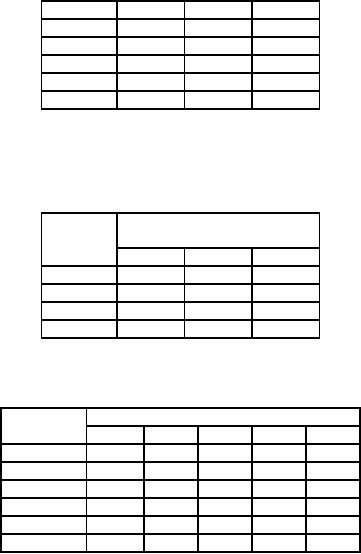
Table
12
Contractor
1
2
3
4
Building
A
4
4
6
0
B
0
4
4
12
C
11
9
5
0
D
0
2
12
4
STEP
2:Choose
the least element in each
column and subtract the same
from all the elements in
that column to
ensure
that there is atleast one
zero in each column. Thus we
have table 13.
Table
13
Contractor
1
2
3
4
Building
A
4
2
2
0
B
2
0x
12
0
C
11
7
1
0x
D
0x
8
4
0
STEP
3:We
make the assignment in each
row and column as explained previously.
This results in table 1
Table
14
Contractor
1
2
3
4
Building
A
4
2
2
0
B
2
0x
12
0
C
11
7
1
0x
D
0x
8
4
0
210
Operations
Research (MTH601)
211
Here
we have only three
assignments. But we must
have four assignments. With this
maximal assignment
we
have to draw the minimum
number of lines to cover all
the zeros. This is carried
out as explained in steps
4
to
9. Refer table 15.
Table
15
Contractor
1
2
3
4
Building
A
4
2
2
0
B
2
0x
12
0
C
11
7
1
0x
D
0x
8
4
0
STEP
4:Mark
(√
)
the unassigned row (row
C).
STEP
5:Against
the marked row C, look
for any 0 element and mark
that column (column 4).
STEP
6:Against
the marked column 4, look
for any assignment and mark
that row (row
A).
STEP
7:Repeat
steps 6 and 7 until the
chain of markings
ends.
STEP
8:Draw
lines through all unmarked
rows (row B and row D) and
through all marked columns
(column 4).
(Check:
There should be only three
lines to cover all the
zeros.)
STEP
9:Select
the minimum from the
elements that do not have a
line through them. In this
example we have 1
as
the minimum element,
subtract the same from
all the elements that do
not have a line through
them and add
this
smallest element at the
intersection of two lines.
Thus we have the matrix
shown in table 16.
Table
16
Contractor
1
2
3
4
Building
A
3
1
1
0
B
2
0x
13
0
C
10
6
0x
0
D
0x
8
5
0
STEP
10:
Go ahead with the assignment
with the usual procedure.
This is carried out in the
table 16. Thus we
have
four assignments.
Building
A is alloted to contractor 4
Building
B is alloted to contractor 1
Building
C is alloted to contractor 3
Building
D is alloted to contractor 2
Total
cost is 44 + 56 + 90 + 44 = Rs. 234
thousands.
An
airline that operates seven
days a week has a timetable
given below. Crews must
have a
Example:
minimum
layover time of 6 hours
between flights. Obtain the
pairing of flights that minimizes
layover time
211
Operations
Research (MTH601)
212
away
from home. For any
given pairing the crew will be
based at the city that
results in the smaller
layover.
For
each pair also mention
the city where the crew
should be placed.
212
Operations
Research (MTH601)
213
Flight
No.
Karachi
to
Islamabad
1
7.00
a.m.
9.00
a.m.
2
9.00
a.m.
11.00
a.m.
3
1.30
p.m.
3.30
p.m.
4
7.30
p.m.
9.30
p.m.
Flight
No.
Islamabad
to Karachi
101
9.00
a.m.
11.00
a.m.
102
10.00
a.m.
12.00
Noon
103
3.30
p.m.
5.30
p.m.
104
8.00
p.m.
10.00
p.m.
Solution:
STEP
1:
We prepare a matrix in which
all the flights reaching
Islamabad are paired with
flights with No's
101,
102,
103 and 104. The
elements in the matrix
represent the time taken
(hrs) by Karachi based crew in
Islamabad.
Refer table 17.
Flight
No.
101
102
103
104
1
24
25
6.5
11
2
22
23
28.5
9
3
17.5
18.5
24
28.5
4
11.5
12.5
18
22.5
Explanation:
The
crew in the first flight No.
1 leaving Karachi arrives at Islamabad at
9.00 a.m. If the crew
is
to
return by flight No. 101, it
is not possible on the same
day and it has to stay
for 24 hours (layover
time).
Similarly
to return by flight No. 102,
103 and 104, the
same crew takes 25 hours,
6.5 hours, 11 hours
respectively.
In the same way we calculate
the time spent by the crew
in flights 2, 3 and 4 to pair
with flights
with
No. 101, 102, 103
and 104. This is shown in Table
17.
STEP
2:We
prepare a matrix in which
all the flights reaching
Karachi are paired with
flights with numbers
1,2,3
and 4. The elements in the
matrix indicate the time
spent by Islamabad based crew in Karachi.
This is
shown
in table 18.
Table
18
Flight
No.
101
102
103
104
1
20
19
13.5
9
2
22
21
15.5
11
3
26.5
25.5
20
15.5
4
8.5
7.5
26
21.5
STEP
3:Comparing
the corresponding elements of
the two matrices (tables 17
and 18), we choose the
minimum
element
and indicate the base at
the top of the element
(Karachi base-D, Islamabad base-C,).
Thus we prepare
the
table 19. If the crew is
placed in either city it is
denoted by *.
213
Operations
Research (MTH601)
214
Table
19
Flight
No.
101
102
103
104
C
C
C
9C
1
20
19
6.5
21C 15.5C
9D
2
22*
17.5D 18.5D
20C 15.5C
3
8.5C 7.5C
18D 21.5C
4
STEP
4:We
proceed with the usual
steps of assignment problem.
Thus we have the following
tables 20 and 21.
Table
20
Flight
No.
101
102
103
104
1
13.5
12.5
0
2.5
2
13
12
6.5
0
3
2
3
5
0
4
1
0
10.5
14
Table
21
Flight
No.
101
102
103
104
1
12.5
12.5
0
25
2
12
12
6.5
0
3
1
3
5
0
4
0
0
10.5
14
We
have the following
assignments shown in table
22. The minimum number of
lines (3), are drawn to
cover all
zero
following Hungarian algorithm.
Table
22
Flight
No.
101
102
103
104
1
12.5
12.5
0
26
√
2
11
11
5.5
0
√
3
0
2
3.5
0
4
0
0
10.5
15
√
STEP
5
Select
the smallest element from
those, which have no lines
through them. In this case
this is 1. Hence
subtract
the
same from all the
elements that do not have a
line through them and
add the same at the
intersection of two
lines.
Thus we have the table
23.
Table
23
Flight
No.
101
102
103
104
1
12.5
12.5
0
26
2
11
11
5.5
0
3
0
2
3.5
0
214
Operations
Research (MTH601)
215
4
0
0
10.5
15
We
assign rowwise and then
columnwise. We have the table
24
Table
24
Flight
No.
101
102
103
104
1
12.5
12.5
26
0
2
11
11
5.5
0
3
2
3.5
0x
0
4
0x
10.5
15
0
The
result can be given
as,
Flight
no. 1 is paired with 103
with base at Karachi.
Flight
no. 2 is paired with 104
with base at Karachi.
Flight
no. 3 is paired with 101
with base at Karachi.
Flight
no. 4 is paired with 102
with base at
Islamabad.
MAXIMIZATION
IN ASSIGNMENT MODEL
The
problem of maximization is carried
out similar to the case of
minization making a slight modification.
The
required
modification is to multiply all
elements in the matrix by
-1, based on the concept
that minizing the
negative
of a function is equivalent to maximize
the original function. This case is illustrated in
the following
example.
Example:
Six
salesmen are to be allocated to
six sales regions. The
earning of each salesman at
each
region
is given below. How can
you find an allocation, so
that the earnings will be
maximum?
Region
Salesman
1
2
3
4
5
6
15
35
0
25
10
45
A
40
5
45
20
15
20
B
25
60
10
65
25
10
C
25
20
35
10
25
60
D
30
70
40
5
40
50
E
10
25
30
40
50
15
F
(Figure
are in Rs. 1000)
In
this problem the objective
is to maximize the earnings of
six salesmen sent to
different
Solution:
regions.
The first step is to
multiply all the elements by
(-1) and apply the
method for minimization. So we
have
the
starting table as shown in
table 25.
Table
25
Region
Salesman
1
2
3
4
5
6
-15
-35
0
-25
-10
-45
A
215
Operations
Research (MTH601)
216
-40
-5
-45
-20
-15
-20
B
-25
-60
-10
-65
-25
-10
C
-25
-20
-35
-10
-25
-60
D
-30
-70
-40
-5
-40
-50
E
-10
-25
-30
-40
-50
-15
F
The
second step is to follow the
procedure of subtracting the
least element from each
row and then in
each
column
to ensure that there is
atleast one zero in each
row and in each column. This is
presented in tables 26
and
27.
Table
26
Region
Salesman
1
2
3
4
5
6
30
10
45
20
35
0
A
5
40
5
25
30
25
B
40
5
55
0
40
55
C
35
40
25
50
35
0
D
40
0
30
65
30
20
E
40
25
20
10
0
35
F
Table
27
Region
Salesman
1
2
3
4
5
6
25
10
45
20
35
0
A
0
40
0
25
30
25
B
35
5
55
0
40
55
C
30
40
25
50
35
0
D
35
0
30
65
30
20
E
35
25
20
10
0
35
F
The
third step is to assign salesmen to
regions and test for
optimality with the usual
method as in table
28.
Table
28
Region
Salesman
1
2
3
4
5
6
25
10
45
20
35
A
0
40
0x
25
30
25
B
0
35
5
55
40
55
C
0
30
40
25
50
35
0x
D
35
30
65
30
20
E
0
35
25
20
10
35
F
0
Since
we have six assignments, we
have an optimal solution as given
below in tables 29 to
31.
216
Operations
Research (MTH601)
217
Salesman
A is assigned to region 1,
B
to region 3,
C
to region 4,
D
to region 6,
E
to region 2 and
F
to region 5
Total
earnings are 15 + 45 + 65 + 60 + 70 + 50 =
Rs. 3.5 (in
thousands)
217
Operations
Research (MTH601)
218
First
iteration
Table
29
Salesman
Region
1
2
3
4
5
6
15
0x
35
10
25
0x
A
40
0x
25
30
35
B
0
35
5
55
40
65
C
0
20
30
15
40
25
D
0
35
30
65
30
30
E
0
35
25
20
10
45
F
0
Table
30
Second
iteration
Salesman
Region
1
2
3
4
5
6
5
0x
25
0x
15
0x
A
50
0x
25
30
45
B
0
35
15
55
40
75
C
0
10
30
5
30
15
D
0
25
30
55
20
30
E
0
35
35
20
10
55
F
0
Table
31
Third
iteration
Salesman
Region
1
2
3
4
5
6
0x
20
5
10
0x
A
0
0x
55
30
30
45
B
0
30
15
50
35
75
C
0
5
30
0x
30
10
D
0
20
15
55
15
30
E
0
35
40
20
15
60
F
0
IMPOSSIBLE
ASSIGNMENT
Sometimes
in an assignment model we are
not able to assign some
jobs to some persons. For
example
if
machines are to be allocated to
locations and if a machine
cannot be accommodated in a particular
location,
then
it i an impossible assignment. To solve
the problem in such
situations we attach a very
highly prohibited
(say
∞)
cost to the cell in the
matrix so that there is
absolutely no chance to get
the assignment with infinite
cost
in
the optimal solution.
218
Operations
Research (MTH601)
219
Example
The
processing times in hours
for the jobs when
allocated to the different machines
are indicated
below.
When a job is not possible to be
made in a particular manner, it is
indicated as '-'
Machine
Jobs
I
II
III
IV
V
3
-
8
-
8
A
4
7
15
18
8
B
8
12
-
-
12
C
5
5
8
3
6
D
10
12
15
10
-
E
Allocate
the machines for the
jobs so that the total
processing time is
minimum.
Solution:
We
have the impossible
assignments marked as -. We introduce
deliberately a high prohibitive
time
(say
∞)
in those places and proceed
with the usual steps of
solution procedure for assignment
problem. Thus we
have
the
table
32.
Table
32
Machine
Jobs
I
II
III
IV
V
∞
∞
8
8
3
A
4
7
15
18
8
B
∞
∞
12
8
12
C
5
5
8
3
6
D
∞
10
12
15
10
E
Reducing
the matrix in rows and
columns so as to have atleast
one zero in each row
and in each
column,
we have the following tables
33 and 34
Table
33
Machine
Jobs
I
II
III
IV
V
∞
∞
8
5
0
A
0
3
11
14
4
B
∞
∞
4
0
4
C
2
2
5
0
3
D
∞
0
2
5
0
E
Table
34
Machine
Jobs
I
II
III
IV
V
∞
∞
0
2
0
A
0
1
6
14
1
B
219
Operations
Research (MTH601)
220
∞
∞
1
0
2
C
2
0
0
0
0
D
∞
0
0
0
0
E
Next
we proceed to assign jobs to
machines as in table
35.
Table
35
Machine
Jobs
I
II
III
IV
V
∞
∞
2
0x
A
0
1
6
14
1
B
0
∞
∞
1
0x
2
C
2
0x
0x
0x
D
0
∞
0x
0x
0x
E
0
From
35 we see that there are
only four assignments but we
should have five
assignments.
We
now proceed with drawing
minimum number of lines to
cover all zeros as in table
36.
Table
36
Machine
Jobs
I
II
III
IV
V
∞
∞
0
2
0x
A
1
6
14
1
B
0
∞
∞
1
0x
2
C
2
0x
0x
0x
D
0
∞
0x
0x
0x
E
0
Now
subtract the least element
from the elements that do
not have a line through
them. In this case this
element
is
1. We subtract it from all
elements, which do not have
a line through them and
add the same at
the
intersection
of two lines. Proceeding in this
way we have the table
37.
Table
37
Machine
Jobs
I
II
III
IV
V
∞
∞
2
1
A
0
0x
5
13
0x
B
0
∞
∞
0
0x
1
C
3
0x
0x
D
0
0
∞
1
0x
0x
E
0
220
Operations
Research (MTH601)
221
(Note:
Since
we have number of zeros
occupying corner of a square, we
have multiple
solutions).
Job
A is assigned to machine III, B to
machine I, C to machine V, D to machine
II, E to machine IV.
221
Operations
Research (MTH601)
222
REVIEW
QUESTIONS
1.
Three
jobs A, B, C are to be assigned to
three machines X, Y, Z. The
processing costs (in Rs.)
are as
given
in the matrix shown below.
Find the allocation, which
will minimize the overall
processing cost.
Machine
jobs
A
B
C
19
28
31
X
11
17
16
Y
12
15
13
Z
2.
A
college department chairman
has the problem of providing
teachers for all courses
offered by his
department
at the highest possible level of
educational 'quality'. He has one
professor, two
associate
professors,
and one teaching assistant
(TA) available. Four courses
must be offered and,
after
appropriate
introspection and evaluation he
has arrived at the following
relative ratings (100 =
basic
rating)
regarding the ability of
each instructor to teach the
four courses, respectively.
Courses
1
2
3
4
Prof.
1
60
40
60
70
Prof.
2
20
60
50
70
Prof.
3
20
30
40
60
T.A.
30
10
30
40
How
should he assign his staff to
the courses to maximize
educational quality in his
department?
3.
(a)
Explain the Hungarian
method of solving an assignment problem
for minimization.
(b)
Solve the following
assignment problem for
minimization with cost (in
rupees) matrix as:
Machine
Jobs
A
B
C
D
E
4
10
3
4
8
1
7
2
6
7
7
2
10
5
8
11
4
3
3
6
5
3
2
4
10
7
3
5
7
5
4.
State
the linear programming formulation of an
assignment problem.
Four
Jobs can be processed on four
different machines, one job on
one
machine.
Resulting profits vary with
assignments. They are
given
below.
Machine
Jobs
A
B
C
D
42
35 28
21
I
222
Operations
Research (MTH601)
223
30
25 20
15
II
30
2
20
15
III
24
20 16
12
IV
Find
the optimum assignment of
jobs to machines and the
corresponding profit.
5.
Five
men are available to do five
different jobs. From past
records the time in hours
that each man
takes
for each job is known
and is given below.
Jobs
Men
I
II
III
IV
V
3
10
3
8
2
A
7
9
8
7
2
B
5
7
6
4
2
C
5
3
8
4
2
D
6
4
10
6
2
E
Find
the assignment of men to
jobs that will minimize
the total time taken.
6.
Pearl
Corporation has four plants
each of which can
manufacture any one of four
products. Production
costs
differ from one plant to
another as do sales revenue. Given
the revenue and cost
data below,
obtain
which product each plant
should produce to minimize
the profit.
Sales
Revenue
Production
Cost
Plant
Product
Product
1
2
3
4
1
2
3
4
50
68
49
62
49
60
45
61
A
60
70
51
74
55
63
45
69
B
55
67
53
70
52
62
49
58
C
58
65
54
69
55
64
48
66
D
7.
Five
different machines can process
any of the five required
jobs with different profits resulting
from
each
assignment.
Machine
Job
A
B
C
D
E
1
130
137
140
128
140
2
140
124
127
121
136
3
140
132
133
-
135
4
-
138
140
136
136
5
129
-
141
134
139
Find
the maximum profit possible
through optimum
assignments.
8.
A
construction company has
five bulldozers at different locations
and one bulldozer is required at
three
different
constructions sites. If the
transportation cost are as
shown, determine the optimum
shipping
schedule.
Shipping
cost ('000 Rs)
Location
Construction
site
223
Operations
Research (MTH601)
224
A
B
C
1
20
30
40
2
70
60
40
3
30
50
80
4
40
60
50
5
40
60
30
9.
A
manager has the problem of
assigning four new machines to three
production facilities.
The
respective
profits derived are as shown. If
only one machine is assigned
to a production facility
determine
the optimal
assignment.
Profits
('000 Rs)
Machine
Production
facility
1
2
3
A
10
10
14
B
10
11
13
C
12
10
10
D
13
12
11
10.
Solve
the following unbalanced
assignment problem of minimizing total
time for doing all
the jobs.
Jobs
Operator
1
2
3
4
5
1
6
2
5
2
6
2
2
5
8
7
7
3
7
8
6
9
8
4
6
2
3
4
5
5
9
3
8
9
7
6
4
7
4
6
8
224
Operations
Research (MTH601)
225
Segment
VII: Queuing Theory
Lectures
38 - 39
225
Table of Contents:
- Introduction:OR APPROACH TO PROBLEM SOLVING, Observation
- Introduction:Model Solution, Implementation of Results
- Introduction:USES OF OPERATIONS RESEARCH, Marketing, Personnel
- PERT / CPM:CONCEPT OF NETWORK, RULES FOR CONSTRUCTION OF NETWORK
- PERT / CPM:DUMMY ACTIVITIES, TO FIND THE CRITICAL PATH
- PERT / CPM:ALGORITHM FOR CRITICAL PATH, Free Slack
- PERT / CPM:Expected length of a critical path, Expected time and Critical path
- PERT / CPM:Expected time and Critical path
- PERT / CPM:RESOURCE SCHEDULING IN NETWORK
- PERT / CPM:Exercises
- Inventory Control:INVENTORY COSTS, INVENTORY MODELS (E.O.Q. MODELS)
- Inventory Control:Purchasing model with shortages
- Inventory Control:Manufacturing model with no shortages
- Inventory Control:Manufacturing model with shortages
- Inventory Control:ORDER QUANTITY WITH PRICE-BREAK
- Inventory Control:SOME DEFINITIONS, Computation of Safety Stock
- Linear Programming:Formulation of the Linear Programming Problem
- Linear Programming:Formulation of the Linear Programming Problem, Decision Variables
- Linear Programming:Model Constraints, Ingredients Mixing
- Linear Programming:VITAMIN CONTRIBUTION, Decision Variables
- Linear Programming:LINEAR PROGRAMMING PROBLEM
- Linear Programming:LIMITATIONS OF LINEAR PROGRAMMING
- Linear Programming:SOLUTION TO LINEAR PROGRAMMING PROBLEMS
- Linear Programming:SIMPLEX METHOD, Simplex Procedure
- Linear Programming:PRESENTATION IN TABULAR FORM - (SIMPLEX TABLE)
- Linear Programming:ARTIFICIAL VARIABLE TECHNIQUE
- Linear Programming:The Two Phase Method, First Iteration
- Linear Programming:VARIANTS OF THE SIMPLEX METHOD
- Linear Programming:Tie for the Leaving Basic Variable (Degeneracy)
- Linear Programming:Multiple or Alternative optimal Solutions
- Transportation Problems:TRANSPORTATION MODEL, Distribution centers
- Transportation Problems:FINDING AN INITIAL BASIC FEASIBLE SOLUTION
- Transportation Problems:MOVING TOWARDS OPTIMALITY
- Transportation Problems:DEGENERACY, Destination
- Transportation Problems:REVIEW QUESTIONS
- Assignment Problems:MATHEMATICAL FORMULATION OF THE PROBLEM
- Assignment Problems:SOLUTION OF AN ASSIGNMENT PROBLEM
- Queuing Theory:DEFINITION OF TERMS IN QUEUEING MODEL
- Queuing Theory:SINGLE-CHANNEL INFINITE-POPULATION MODEL
- Replacement Models:REPLACEMENT OF ITEMS WITH GRADUAL DETERIORATION
- Replacement Models:ITEMS DETERIORATING WITH TIME VALUE OF MONEY
- Dynamic Programming:FEATURES CHARECTERIZING DYNAMIC PROGRAMMING PROBLEMS
- Dynamic Programming:Analysis of the Result, One Stage Problem
- Miscellaneous:SEQUENCING, PROCESSING n JOBS THROUGH TWO MACHINES
- Miscellaneous:METHODS OF INTEGER PROGRAMMING SOLUTION