A Firm’s Short-Run Costs ($):The Effect of Effluent Fees on Firms’ Input Choices

<< Measuring Cost: Which Costs Matter?:Cost in the Short Run

Cost in the Long Run:Long-Run Cost with Economies & Diseconomies of Scale >>

Microeconomics ECO402

Lesson 19

A Firm's Short-Run Costs ($)

Rate

Fixed

Variable Total

Marginal Average

Average

cost

fixed

variable

total

output FC

cost

AFC

AVC

ATC

100

128

148

16.5

32.7

49.3

112

162

12.5

40.5

130

180

150

200

8.3

33.3

175

225

7.1

32.1

204

254

6.3

25.5

31.8

242

292

5.6

26.9

32.4

300

350

385

435

4.5

39.5

Consequently (from the table):

MC decreases initially with increasing returns

· 0 through 4 units of output

MC increases with decreasing returns

· 5 through 11 units of output

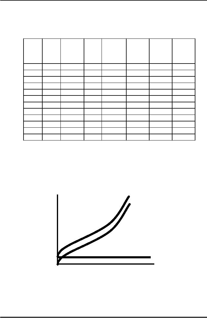
Total cost

is the vertical

Cost

sum of FC

($ per 400

and VC.

year)

Variable cost

increases with

300

production and

the rate varies with

increasing &

decreasing returns.

200

Fixed cost does not

100

vary with output

Output

Microeconomics ECO402

Cost 100

($ per

unit)

ATC

AVC

AFC

Output (units/yr.)

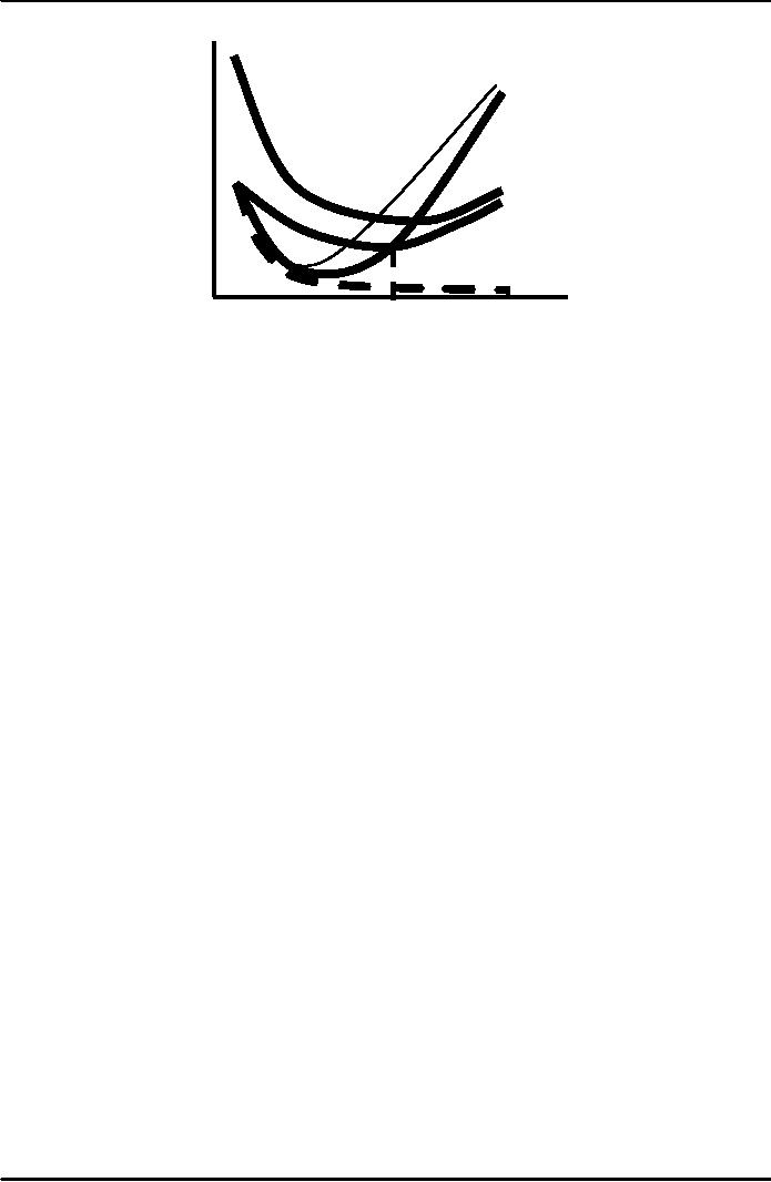
The line drawn from the origin to the tangent of the variable cost curve:

Its slope equals AVC

The slope of a point on VC equals MC

Therefore, MC = AVC at 7 units of output (point A)

Unit Costs

AFC falls continuously

When MC < AVC or MC < ATC, AVC & ATC decrease

When MC > AVC or MC > ATC, AVC & ATC increase

MC = AVC and ATC at minimum AVC and ATC

Minimum AVC occurs at a lower output than minimum ATC due to FC

The User Cost of Capital

User Cost of Capital = Economic Depreciation + (Interest Rate)(Value of Capital)

Example

· An Airline buys a Boeing 737 for $150 million with an expected life of 30 years

Annual economic depreciation = $150 million/30 = $5 million

Interest rate = 10%

· User Cost of Capital = $5 million + (.10) ($150 million depreciation)

Year 1 = $5 million + (.10)($150 million) = $20 million

Year 10 = $5 million + (.10) ($100 million) = $15 million

Rate per dollar of capital

· r = Depreciation Rate + Interest Rate

Airline Example

· Depreciation Rate = 1/30 = 3.33/yr

· Rate of Return = 10%/yr

User Cost of Capital

· r = 3.33 + 10 = 13.33%/yr

Microeconomics ECO402

The Cost Minimizing Input Choice

Assumptions

· Two Inputs: Labor (L) & capital (K)

· Price of labor: wage rate (w)

· The price of capital

R = depreciation rate + interest rate

Question

· If capital was rented, would it change the value of r ?

The Isocost Line

C = wL + rK

Isocost: A line showing all combinations of L & K that can be purchased for the same

cost

Rewriting C as linear:

· K = C/r - (w/r)L

· Slope of the Isocost:

()

ΔK

=- w

ΔL

is the ratio of the wage rate to rental cost of capital.

This shows the rate at which capital can be substituted for labor with no

change in cost.

Choosing Inputs

· We will address how to minimize cost for a given level of output.

· We will do so by combining Isocosts with Isoquants

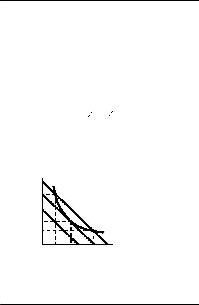
Producing a Given Output at Minimum Cost

Q1 is an isoquant

Capital

for output Q1.

per

Isocost curve C0 shows

year

all combinations of K and L

that can not produce Q1 at

this

Isocost C2 shows quantity

CO C1 C2 are

Q1 can be produced with

three

combination K2L2 or K3L3.

Isocost lines

However, both of these

are higher cost combinations

than K1L1.

Labor per year

Microeconomics ECO402

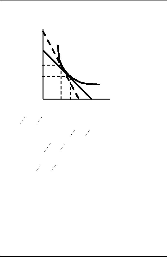
Input Substitution When an Input Price Change

Isoquants and Isocosts and the Production Function

Capital

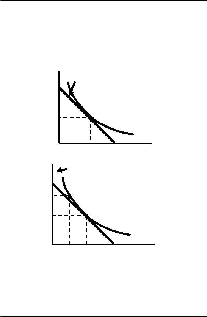
If the price of labor

changes, the Isocost curve

per

becomes steeper due to

year

the change in the slope -(w/L).

This yields a new combination

of K and L to produce Q1.

Combination B is used in place

of combination A.

The new combination represents

the higher cost of labor relative

to capital and therefore capital

is substituted for labor.

Labor per year

MRTS = -ΔK

= MPL

ΔL

MPK

Slope of isocost line = ΔK

= -w

ΔL

MPL

and =

MPK

The minimum cost combination can then be written as:

MPL

= MPK

Minimum cost for a given output will occur when each dollar of input added to the

production process will add an equivalent amount of output.

Question

If w = $10, r = $2, and MPL = MPK, which input would the producer use more of? Why?

The Effect of Effluent Fees on Firms' Input Choices

Firms that have a by-product to production produce an effluent.

An effluent fee is a per-unit fee that firms must pay for the effluent that they emit.

How would a producer respond to an effluent fee on production?

The Scenario: Steel Producer

Microeconomics ECO402

1) Located on a river: Low cost transportation and emission disposal

(effluent).

2) EPA imposes a per unit effluent fee to reduce the environmentally harmful

effluent.

3) How should the firm respond?

The Cost-Minimizing Response to an Effluent Fee

Capital

(machine

Slope of

hours per

Isocost = -10/40

5,000

month)

= -0.25

4,000

3,000

2,000

Output of 2,000

1,000

Tons of Steel per Month

Waste Water

5,000

10,000 12,000 18,000

20,000

(gal./month)

Capital

(machine

Prior to regulation the

Slope of

hours per

firm chooses to produce

Isocost = -

month)

an output using 10,000

20/40

5,000

gallons of water and 2,000

= -0.50

machine-hours of capital at A.

4,000

Following the imposition

of the effluent fee of $10/gallon

3,500

the slope of the Isocost changes

3,000

which the higher cost of water to

capital so now combination B

is selected.

2,000

1,000

Output of 2,000

Tons of Steel per Month

Waste Water

5,000

(gal./month)

10,000 12,000 18,000

20,000

Observations:

The more easily factors can be substituted; the more effective the fee is in reducing the

effluent.

The greater the degree of substitutes, the less the firm will have to pay (e.g.: $50,000 with

combination B instead of $100,000 with combination A).

Table of Contents: