 |
Transportation Problems:MOVING TOWARDS OPTIMALITY |
| << Transportation Problems:FINDING AN INITIAL BASIC FEASIBLE SOLUTION |
| Transportation Problems:DEGENERACY, Destination >> |
Operations
Research (MTH601)
176
MOVING
TOWARDS OPTIMALITY
The
rationale behind
optimality
Given
an initial non-degenerate basic
feasible solution, a question
may arise as to how we can
find a
successively
better basic feasible
solution. This means that we
have to select an entering
variable, a leaving
basic
variable and identify the
corresponding solution. In the
transportation model, selecting an
entering variable
means
selecting a new cell in which to
make a non-zero allocation in the
transportation matrix. The principle
of
selecting
the variable which improves
the value of the objective
function (minimizes the total
transportation
cost),
at the fastest rate is still
valid. So we select an unoccupied
cell and make a unit
allotment, so that the
cost
of
transportation will decrease by
the greatest amount.
To
illustrate, suppose that in the
example 4.1 we choose arbitrarily
the cell (B, P) which is
unoccupied
and
make + 1 allotment in this cell. This new allocation automatically
violates the supply
situation and demand
requirements
of the origin B and
destination P. So changes are
required in other cells to
restore feasibility. This
necessitates
a reallocation in the cells to
restore feasibility. This necessitates a
reallocation in the cells
(B, P),
(A,
P), (A, Q) and (B,
Q). The row total and column
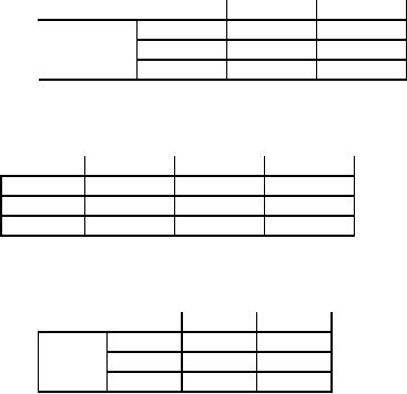
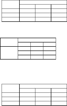
total will be unaltered. This idea is
illustrated in tables 17 to
19.
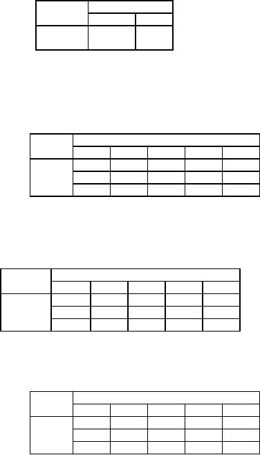
Table
17
P
Q
R
A
5
7
8
B
4
4
6
C
6
7
7
Unit
cost of transportation
Table
18
P
Q
R
A
65
5
70
B
30
30
C
7
43
50
65
42
43
Table
19
P
Q
R
A
65-1
5+1
70
B
1
30-1
30
C
7
43
50
65
42
43
Changed
allotment
The
unit costs in the cells
(B, P), (A, P),
(A, Q) and (B, Q) are 4, 5,
7, 4 respectively (refer table
17).
The
total change in the total cost
will be 4 - 5 + 7 - 4 = + 2. We see that
this arbitrary unit allotment to cell
(B,
P)
increases the transportation
cost by rupees 2. Hence an allocation to
the cell (B, P) is not
recommended.
This
procedure is repeated by choosing
some other unoccupied cell
for allocation. This
requires
corresponding
changes in the allocation in the
occupied cells to restore
feasibility and calculation of
the
176
Operations
Research (MTH601)
177
marginal
cost. If, by this procedure,
we get a +ve
value,
it indicates that the total
cost is not decreasing
but
increasing.
Consider
the objective function to
minimize,
mn
Z=∑∑
c
x
ij
ij
i
=1
j
=1
and
the restrictions as
n
0
=
ai - ∑ xij for
i
=
1,2, ...
,
m
j
=1
m
0
=
b
-
∑ xij for
j = 1,2, ...
,
n
j
i
=1
Multiply
each of these equations by a
number and add this
multiple to the objective function.
This resultant can
be
used to eliminate the basic
variable. Let us represent the
multiples by ui (i =
1, 2, ..., m)
and vj =
(j
=
1, 2, ...,
n)
respectively for rows and
columns. These multipliers
are called the simplex
multipliers.
Therefore,
⎡
⎤
m
m
n
n
+
∑ ui ⎢
ai - ∑
xij ⎥
Z
=
∑ ∑ cij
x
i
=1
⎢
⎥
ij
i
=1
j
=1
⎣
j
=1
⎦
⎡
⎤
n
m
+
∑ v
j ⎢b j - ∑
xij ⎥
⎢
i
=1
⎥
⎣
⎦
j
=1
m
m
n
n
(
)
=
∑ ∑ cij -ui -v j x
+ ∑
ui ai
+
∑ v
j b j
ij
i
=1
j
=1
i
=1
i
=1
Thus
in order to have a zero coefficient
(for a basic variable) it is
necessary that
crs =
ur +
vs
for
each basic variable
xrs (i.e.)
for each occupied cell
(r,
s).
There are (m
+ n - 1)
occupied cells and
therefore
(m + n
-
1) equations. Since we have
(m
+ n) unknown
(ui's
and
vj's)
one of these variables can
be assigned a
177
Operations
Research (MTH601)
178
value
arbitrarily and rest of them
can then be solved algebraically. This
leads to the solution of a set of (m
+
n
- 1) equations simultaneously.
Having
determined the values of
ui and
vj,
the entering basic variable
(if any) can be identified
readily
by
calculating cij -
(ui +
vj) for
each of the unoccupied
cells. If cij -
(ui +
vj) > 0 in
every case, then the
solution
must
be optimal since no non-basic
variable can decrease
Z.
On the other hand if
cij -
(ui +
vj)
yields a negative
result,
the cell with the
largest negative (smallest)
value of cij -
(ui +
vj) is
selected to be the cell for
new
allocation
since it means that this
non-basic variable decreases Z at
the fastest rate. This is
the basis for
conducting
the optimality test, which
is explained in the next
section.
Optimality
test:
For
conducting the optimality
test to any feasible solution of a
(mxn)
transportation problem,
the
following
two conditions must be
satisfied.
1.
It
consists of exactly
(m + n
-
1) individual cells being
allocated.
2.
These
allocations are in independent
positions.
The
first condition is normally satisfied in
many problems. If the first
condition is not satisfied then it
results in
a
state known as degeneracy, in
the transportation mode. The
discussion of degeneracy and
its resolution is
explained
in a later section.
A
set of allocations comprising a feasible
solution is said to be in 'independent
positions' if it is
impossible
to increase or decrease any
individual allocation without either
changing the positions of
allocations
or
violating the row or column
restrictions. In other words, a simple criterion
for independence is that, it
is
impossible
to travel from any allocation
back to itself, by a series of
alternating horizontal and vertical
jumps
from
one occupied cell to
another, without a direct
reversal of route.
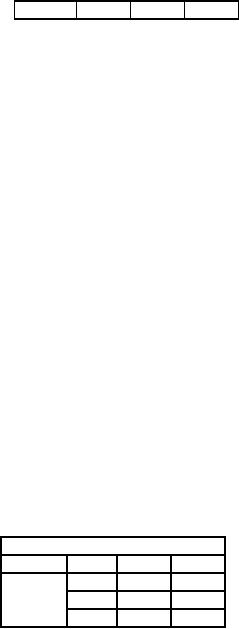
For
example, if the occupied cells
form a closed loop as in
table 20 they are not in
independent
positions
Table
20
*
*
*
*
Applying
the procedure outlined above
to the initial basic
feasible solution, (found by
any method) we have
the
following
steps in conducting an optimality
test.
STEP
1:Write
the matrix of allotment found by
NWC rule or by Vogel's Approximation
Method. Check for
conditions
for optimality (i.e.) there
must be (m + n - 1) alloted cells
and all of them must be in
independent
positions.
If these two conditions are
satisfied, proceed to step
2.
STEP
2:Write
the matrix of the cost of
the alloted cells.
STEP
3:Determine
a set of (m
+ n)
numbers,
ui,
i
=
1, 2, ..., m
vj,
j
=
1, 2, ..., n
178
Operations
Research (MTH601)
179
called
simplex multipliers such
that for each occupied
cell (r, s).
crs =
ur + vs
where
crs is
the individual cost of an allocation
from origin r
to
destinations s.
This
can be done by arbitrarily
assigning, any one of the
ui's
or
vj's,
any value (say 0) and
satisfying the above
equation
for all the occupied
cells.
STEP
4:Write
the matrix of cost elements
for all unoccupied
cells.
STEP
5:Find
(ur +
vs) for
each unoccupied cell and
form the matrix of
(ui +
vj) for
each of the unoccupied
cell.
STEP
6:Calculate
cij -
(ui +
vj) for
each of the unoccupied
cells. This is the matrix of
cell evaluation or square
evaluation.
If the value of cell
evaluation is positive, it indicates that
the solution already found is optimal. If
it
is
negative there is a scope
for relocation of items so
that the total cost of
transportation can be made
minimum.
If
there are many negative
entries in the matrix of
cell evaluation, select the
cell yielding the most
negative entry
as
the entering variable. This
requires reallotment of the allocation
matrix. By including this cell
for occupation,
the
allocations of the other
occupied cells require a
revision to fulfill the row
and column restrictions. If
the
value
of cell evaluation is zero,
then this indicates that
there exists another solution to
the transportation
problem
without
reducing the total
cost.
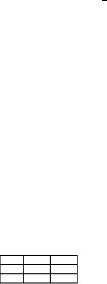
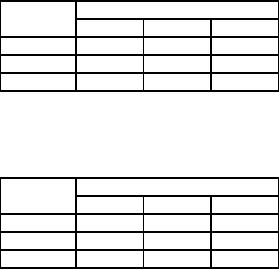
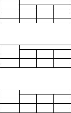
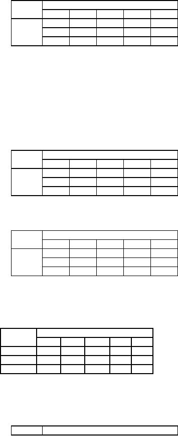
Consider
the example whose cost
matrix is as in table 21
Table
21
Origin
Destination
Supply
P
Q
R
A
5
7
8
70
B
4
4
6
30
Cost
Matrix
C
6
7
7
50
Demand
65
42
43
We
have the allocation as per
NWC rule as in table
22
Table
22
Origin
Destination
Supply
P
Q
R
A
65
5
70
B
30
30
Allotment
Matrix
C
7
43
50
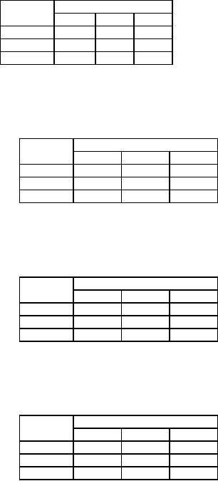
Next
we write the matrix of the
cost of alloted cells and
using explained below and
shown in table 23
Table
23
179
Operations
Research (MTH601)
180
ui
Origin
Destination
P
Q
R
A
5
7
-
0
u1
B
-
4
-
-3
Finding
ui,
vj using
the
u2
C
0
cost
of the occupied cells
-
7
7
u3
vj
v1
v2
v3
5
7
7
To
determine ui's
and
vj's
we arbitrarily
assign one of the
multipliers say u3 the
value 0.
Then
it follows that v2 = 7 because we have the
equation
u3 +
v2 = 7
Since
u3 +
v3 = 7
we
have
v3 = 7
Similarly
using the cost elements of
the occupied cells and
with the equation crs =
ur + vs, we
can find
the
values of ui's
and
vj's.
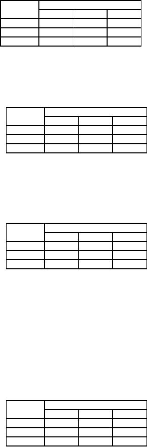
The
unoccupied (un-allotted) cells
are indicated by placing
dots in the cells.
Next
we write the matrix of the
cost elements cij of
the unoccupied cells as in
table 24.
Table
24
Origin
Destination
P
Q
R
A
8
B
4
6
cost
of
C
6
unoccupied
cells
Next
we write the matrix of
ui + vj
for
unoccupied cells as in
Table
25
Origin
Destination
P
Q
R
A
7
B
2
4
(ui +
vj)
for
C
5
unoccupied
cells
Table
26
Origin
Destination
P
Q
R
A
1
B
2
2
Cell
Evaluation
180
Operations
Research (MTH601)
181
C
1
Next
we write the matrix of
ui +
vj for
unoccupied cells as in table
25. Next we find cij -
(ui +
vj) for
all
the
unoccupied cells. This
matrix is obtained by subtracting
the elements in the
(ui +
vj)
matrix from the
corresponding
elements of cij in
the matrix of the cost of
unoccupied cells. This is the
matrix of cell evaluation
or
square evaluation as shown in
table 26.
We
see that all the
elements of the matrix of
cell evaluation are positive
(>
0).
This indicates that
our
initial
basic solution is optimal and
the cost of transportation is
Rs. 830. If the elements of
matrix of cell
evaluation
are negative, it indicates
that further reduction in
cost is possible.
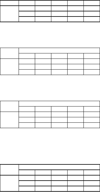
Example
Mam
enterprise has three
factories located at A, B and C
and supplies to three
warehouses located at D,
E
and F. Monthly factory capacities
are 10, 80 and 15 units
respectively. Monthly warehouse
requirements are
45,
20 and 40 units respectively.
Unit transportation costs in
rupees are given
below.
Warehouse
Factory
D
E
F
A
5
1
7
B
6
4
6
C
3
2
5
Starting
with NWC rule, find
the optimal allotment.
Solution:
Using
NWC rule we obtain the
initial basic feasible solution as in
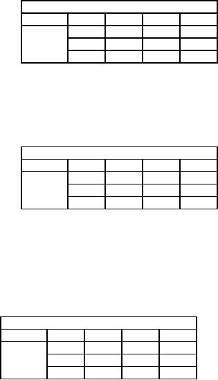
table 27.
Table
27
Warehouse
Factory
D
E
F
Supply
A
10
10
0
B
35
20
25
80
45
25
0
C
15
15
0
45
20
40
35
15
0
0
0
There
are five allotments. As per
the optimality test
conditions there must be (3 + 3 - 1)
cells occupied
and
we see that this condition is
satisfied. Secondly all the
cells should be in independent
positions.
To
test the cells whether
they are independent or not,
we take an occupied cell and
alter the allotment in
that
cell by one unit. This requires
the change in other occupied
cells without violating the
constraints. Or if we
start
from one occupied cell
and we do come back to the
starting cell, then the
cells are in dependent
positions.
In
the above problem all
the cells are
independent.
Having
satisfied the two conditions
we proceed to the optimality
test as described above and
are carried
in
tables 28 to 33
Table
28
181
Operations
Research (MTH601)
182
Factory
Warehouse
D
E
F
A
5
1
7
B
6
4
6
C
3
2
5
Cost
Matrix
Table
29
Factory
Warehouse
D
E
F
A
10
B
35
20
25
C
15
Allotment
Matrix
182
Operations
Research (MTH601)
183
Table
30
Factory
Warehouse
ui
D
E
F
A
5
-
-
0
u1
B
6
4
6
1
u2
C
-
-
5
0
u3
vj
v1
v2
v3
5
3
5
Evaluation
ui and
vj
Table
31
Factory
Warehouse
D
E
F
A
1
7
B
C
3
2
Cost
of un-allotted cells
Table
32
Factory
Warehouse
D
E
F
A
3
5
B
C
5
3
(u1 +
vj) for
un-allotted cells
Table
33
Factory
Warehouse
D
E
F
A
-2
2
B
C
-2
-1
Cell
Evaluation
In
the matrix of cell
evaluation, there are three
cells (A, E), (C, D), and
(C, E) having negative
entries
indicating
the scope of minimizing the
cost by bringing any of these
cells for occupation. But
the most negative
element
is found in two cells (A, E)
and (C, D). Since
there is a tie, the same is
broken arbitrarily. We select
the
cell
(C, D) for reallotment (as
marked in table 34). With
the initial feasible
solution,
Table
34
183
Operations
Research (MTH601)
184
Warehouse
Factory
D
E
F
A
10
B
35
20
25
C
15
we
have to allocate as much as
possible in the empty cell
(with the mark) with the
most negative evaluation
to
arrive
at the minimum cost as
quickly as possible. The
reallocation is performed by identifying
the loop joining
the
empty cell to the occupied
cells by horizontal and vertical jumps as
indicated in table
35.
Table
35
Factory
Warehouse
D
E
F
A
10
B
35
20
25
C
15
It
can be seen that we can
allocate 15 units to cell
(C, D) and still satisfy
the row and column total
and
thus
no allocation becomes negative. The
effect of allotting 15 units to
empty cell leads to the
matrix of
reallotment
as shown in table 36.
Table
36
Factory
Warehouse
D
E
F
A
10
B
20
20
40
C
15
Reallotment
among cells of loop
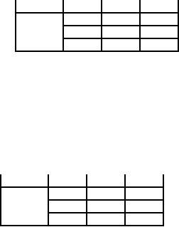
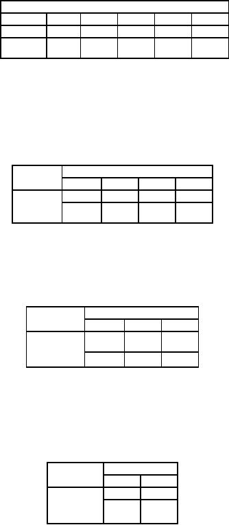
We
conduct optimality test to
see whether this solution is optimal.
The computations are carried
in
tables
37 to 42. From the table 42
we see that the unoccupied
cell (A, E) has a negative
evaluation and hence
there
exists another feasible solution as
shown in table 4
We
have to conduct the
optimality test to find
whether the third feasible solution is
optimal. By
carrying
out the iterations (not
shown), we observe that the
third feasible solution (Table 43) is
optimal and the
corresponding
cost is
10
×
1
+
30
×
6
+
10
×
4
+
40
×
6
+
15
×
3
=
Rs.
515.
Table
37
Factory
Warehouse
D
E
F
A
5
1
7
B
6
4
6
C
3
2
5
184
Operations
Research (MTH601)
185
Cost
Matrix
Table
38
Factory
Warehouse
D
E
F
A
10
B
20
20
40
C
15
Allotment
Matrix
Table
39
Factory
Warehouse
ui
D
E
F
A
5
-1
B
6
4
6
0
C
3
-3
6
4
6
vj
Cost
of alloted cells & Evaluation of
ui and
vj
Table
40
Factory
Warehouse
D
E
F
A
1
7
B
C
2
5
Cost
of unalloted cells
185
Operations
Research (MTH601)
186
Table
41
Factory
Warehouse
D
E
F
A
3
5
B
C
1
3
(ui +
vj)
for unalloted cells
Table
42
Factory
Warehouse
D
E
F
A
-2
2
B
C
1
2
Cell
Evaluation
Table
43
Factory
Warehouse
D
E
F
A
10
B
30
10
40
C
15
Reallotment
Vogel's
Approximation Method for
maximization problem
The
VAM method can be used in a
maximization problem making a slight
modification. The
required
modification
is to multiply all the
elements in the (profit)
matrix by -1, with the
concept that minimizing
the
negative
of a function maximizes the original
function.
Consider
the example given
below.
186
Operations
Research (MTH601)
187
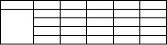
Example:
Solve
the following transportation
problem to maximize profit
and give criteria for
optimality.
Profits
(Rs) / Unit
Destination
Origin
1
2
3
4
Supply
A
40
25
22
33
100
B
44
35
30
30
30
C
38
38
28
30
70
Demand
40
20
60
30
We
first convert the elements
of profit matrix by multiplying by -1
and then we adopt
the
Solution:
method
of minimization. This is done in
table 44
Table
44
Destination
Origin
1
2
3
4
Supply
A
-40
-25
-22
-33
100
B
-44
-35
-30
-30
30
C
-38
-38
-28
-30
70
Demand
40
20
60
30
In
the above problem total
supply is not equal to total
demand. (supply demand) and
hence it is an
unbalanced
transportation model. To balance, we
introduce a dummy column 5. to find
the initial feasible
solution
by VAM. We put the elements in
the dummy column 90 as in table
45
Table
45
Destination
Origin
1
2
3
4
Supply
(Penalty
A
-40
-25
-22
-33
100
(7)
B
-44
-35
-30
-30
30
(9)
C
-38
-38
-28
-30
70
(0)
Demand
40
20
60
30
Penalty
(4)
(3)
(2)
(3)
Allot
in the row B having maximum
penalty and in the cell
(B, I) with least
cost.
The
origin B is deleted for
further analysis as it is exhausted. We
have the reduced matrix
given in table
46.
187
Operations
Research (MTH601)
188
Table
46
Destination
Origin
1
2
3
4
5
Supply
Penalty
A
-40
-25
100
(7)
20
-28
-30
0
70
(0)
C
-38
-38
Demand
10
20
60
30
50
Penalty
(2)
(13)
(6)
(3)
(0)
Allot
in the column (2), which has
a maximum penalty (13) and
in the cell (C, 2) with
least cost. Column 2 is
deleted
as the supply is satisfied
and we have the reduced
matrix as in table 46
Table
47
Origin
Destination
Supply
Penalty
1
3
4
5
A
-40
-22
-33
0
C
10
-28
-30
0
100
(7)
-38
Demand
10
60
30
0
50
(8)
Penalty
(2)
(6)
(3)
(0)
Allot
(C, 1) with 10 units and
delete column 1. Then we have
table 48
Table
48
Origin
Destination
Supply
Penalty
3
4
5
30
0
100
(11)
A
-22
-33
-28
-30
0
40
(2)
C
Demand
60
30
50
Penalty
(6)
(3)
(0)
Allot
30 to cell (A, 4) and delete
column 4. Then we have table
49
Table
49
Origin
Destination
Supply
Penalty
3
5
A
-22
0
70
(22)
40
-28
C
0
40
(28)
Demand
60
50
Penalty
(6)
(0)
Deleting
row C we have the table 50
as we allot 40 to cell (C,
3).
Table
50
188
Operations
Research (MTH601)
189
Destination
Supply
Origin
3
5
50
20
0
-22
70
A
Demand
20
50
Thus
we have the initial feasible
solution given in table 51
Table
51
Origin
Destination
1
2
3
4
5
A
20
30
50
B
C
10
20
40
Allotment
Matrix
The
optimality test is conducted
table 52 to 55
Table
52
Origin
Destination
1
2
3
4
5
ui
A
-
-
-22
-30
0
6
B
-44
-
-
-
-
-6
C
-38
-38
-28
-
-
0
-38
-38
-28
-36
-6
vj
Evaluation
of ui's
and
vj's
Table
53
Origin
Destination
1
2
3
4
5
A
-40
-25
B
-35
-30
-30
0
C
-30
0
Cost
of un-allotted cells
189
Operations
Research (MTH601)
190
Table
54
Origin
Destination
1
2
3
4
5
A
-32
-32
B
-44
-34
-42
-12
C
-36
-6
(ui +
vj) for
unalloted cells
From
table 55 see that the
cell (A, 1) has a negative
value indicating that there is
scope for optimality.
This
is a potential box to be alloted.
Therefore we go back to the allotment
matrix in table 51.
Allotting to cell
(A,
1) we have to remove from
cell (A, 3), add to
cell (C, 3) and remove
from cell (C, 1) so that
the loop is
complete
indicating that reallotment is possible.
Now we have to decide the
amount to be alloted and this
is
decided
with the idea that in
the process of reallotment no
cell can have negative
allotment. Hence we have
the
new
allotment as per the following
table 56
Table
55
Origin
Destination
1
2
3
4
5
A
-8
-7
B
9
4
12
12
C
6
6
Cell
Evaluation
Table
56
Origin
Destination
1
2
3
4
5
A
10
10
30
50
B
30
C
20
50
Reallotment
Table
57
Origin
Destination
ui
1
2
3
4
5
A
-40
-
-22
-33
0
0
B
-44
-
-
-
-
-4
C
-38
-28
-
-
-6
-40
-32
-22
-33
0
vj
Evaluation
of ui and
vj
Table
58
Origin
Destination
190
Operations
Research (MTH601)
191
1
2
3
4
5
A
-25
B
-35
-30
-30
0
C
-38
-30
0
Cost
of unalloted cells
Table
59
Origin
Destination
1
2
3
4
5
A
-32
B
-36
-26
-37
-4
C
-46
-39
-6
(ui +
vj) for
unalloted cells
Table
60
Origin
Destination
1
2
3
4
5
A
7
B
1
-4
7
4
C
8
9
6
Cell
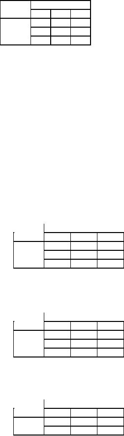
Evaluation
The
matrix of cell evaluation of
cell evaluation in table 60
shows a negative entry in
the cell (B, 3)
indicating
that this is a potential
cell for allotment so that we
get a better result. Hence
we make a reallotment as
shown
by dotted lines in table
61.
Table
61
Origin
Destination
1
2
3
4
5
A
20
30
50
B
20
10
C
20
50
Reallotment
We
can conduct once again
the optimality test. One
more iteration would reveal
that the allotments
in
the
table 61 are optimal. This iteration is
left to the reader. Hence
the profit
=
(20
×
40)
+
(30
×
33)
+
(20
×
44)
+
(50
×
0)
+
(10
×
30)
+
(20
×
38)
+
(50
×
20)
=
Rs.5130.
191
Operations
Research (MTH601)
192
REVIEW
QUESTIONS
1.
Solve
the following transportation
problem for minimization
(Unit costs are given in
rupees).
Destination
Origin
D1
D2
D3
D4
D5
Supply
01
4
3
1
2
6
40
02
5
2
3
4
5
30
03
3
5
6
3
2
20
04
2
4
4
5
3
10
Demand
30
30
15
20
5
2.
A
manufacturer has distribution centres at
X, Y and Z. These centres
have availability of 40, 20
and 40
units
of the product, His retail
outlets at A, B, C, D and E require
25, 10, 20, 30 and 15
units
respectively.
The transport cost per
unit between each centre
and each outlet is given
below.
Retail
Outlets
Distribution
A
B
C
D
E
Centre
X
55
30
40
50
50
Y
35
30
100
45
60
Z
40
60
95
35
30
Determine
the optimal distribution to minimize
the cost of
transportation.
3.
(a)
A company has three
warehouses, W1,
W2 and
W3 and
four retail stores S1, S2,
S3 and
S4.
The
availability
of a given commodity at these
warehouses are as follows:
W1 = 14,
W2 = 16,
W3 = 5.
The
demands
at these stores are:
S1 = 6,
S2 = 10,
S3 = 15,
S4 = 4.
The costs of transporting
one unit of the
commodity
from warehouse i to store j, in
rupees, are given in the
following table.
S1
S2
S3
S4
6
4
1
5
W1
8
9
2
7
W2
4
3
6
2
W3
Determine
the optimum transportation
schedule, which minimizes
the total transportation
cost.
4.
A
firm manufacturing a single
product has three plants at
locations X,
Y and
Z.
The three plants
have
produced
60, 35 and 40 units
respectively during the
week. The firm has
made commitments to sell 22,
45,
20, 18 and 30 units of the
product to customers A,
B, C, D and
E
respectively.
The net per unit
cost
of
transporting from the three
plants to the five customers
is given in the table
below.
192
Operations
Research (MTH601)
193
Customers
Plant
Locations
A
B
C
D
E
X
4
1
3
4
4
Y
2
3
2
2
3
Z
3
5
2
4
4
Use
Vogel's approximation method to determine
the cost of shifting the
product from plant locations
to
the
customers. Does your
solution provide a least
cost transportation
schedule?
5.
A
steel company has three
furnaces and five rolling
mills. Transportation costs
(Rupees per quintal)
for
sending
steel from furnaces to
rolling mills are given in
the following table.
Rolling
Mills
Furnaces
M1
M2
M3
M4
M5
Availability
A
4
2
3
2
6
8
B
5
4
5
2
1
12
C
6
5
4
7
3
14
Required
4
4
10
8
8
How
should they meet the
requirement?
6.
A
company has three factories
at A, B and C, which supply
warehouses at D, E, F and G
respectively.
Monthly
product capacities of these
factories are 250, 300
and 400 units respectively.
The current
warehouse
requirements are 200, 275
and 300 units respectively.
Unit transportation costs
from
factories
to warehouses are given
below.
To
D
E
F
G
A
11
13
17
14
B
16
18
14
10
C
21
24
13
10
Determine
the optimum distribution to minimize
cost.
7.
Solve
the following transportation
problem for minimization,
the cost matrix is given
as:
D1
D2
D3
D4
D5
ai
01
12
4
9
5
9
55
02
8
1
6
6
7
45
03
1
12
4
7
7
30
04
10
15
6
9
1
50
40
20
50
30
40
b1
Find
all the alternate optimal
solutions.
8.
Solve
the following transportation
problem for
minimization.
To
I
II
III
IV
V
ai
20
19
14
23
16
40
A
193
Operations
Research (MTH601)
194
15
20
13
19
16
60
B
18
15
18
20
100
70
C
30
40
50
40
60
bj
9.
Pir
Iron and Steel Company
(PISCO) has three open
hearth furnaces and five
rolling mills.
Transportation
costs (Rs. per quintal) for
shipping steel from furnaces
to rolling mills are shown
in the
following
table.
Mills
Furnaces
M1
M2
M3
M4
M5
Capacities
4
2
3
2
6
8
F1
5
4
5
2
1
12
F2
6
5
4
7
7
14
F3
Required
4
4
10
8
8
What
is an optimal shipping schedule
for PISCO?
10.
A
company having plants at
P,
Q and
R
supplies
to the warehouses at W,
X, Y and
Z.
Monthly plant
capacities
are 75, 95, and
120 respectively. Monthly
warehouse requirements are
55, 65, 75 and
100
respectively.
Unit shipping costs are as
follows.
W
X
Y
Z
P
18
21
15
12
Q
16
22
26
15
R
16
15
16
17
Determine
the optimum distribution for
this company to minimize the
shipping costs using VAM
for
initial
solution.
11.
The
Products of three plants
F1,
F2 and
F3 are
to be transported to 5 warehouses
W1, W2,
W3, W4
and
W5. The
capacities of plants, the
requirements of ware houses
and the cost of
transportation are
indicated
in the following
table.
W1
W2
W3
W4
W5
Plant
Capacity
74
56
54
62
68
400
F1
58
64
62
58
54
500
F2
66
70
52
60
60
600
F3
Demand
200
280
240
360
320
Find
the optimum transportation
schedule and the associated
cost of transportation.
12.
Goods
are to be transported from
three warehouses to six
customers. The availabilities at
the
warehouses
are 100, 120 and
150 units respectively. The
demands of customers are 50,
40, 50, 90, 60
and
80 respectively. The unit
transportation costs are
given in the following
table.
C1
C2
C3
C4
C5
C6
15
25
18
35
40
26
W1
22
36
40
60
50
38
W2
26
38
45
52
45
48
W3
194
Table of Contents:
- Introduction:OR APPROACH TO PROBLEM SOLVING, Observation
- Introduction:Model Solution, Implementation of Results
- Introduction:USES OF OPERATIONS RESEARCH, Marketing, Personnel
- PERT / CPM:CONCEPT OF NETWORK, RULES FOR CONSTRUCTION OF NETWORK
- PERT / CPM:DUMMY ACTIVITIES, TO FIND THE CRITICAL PATH
- PERT / CPM:ALGORITHM FOR CRITICAL PATH, Free Slack
- PERT / CPM:Expected length of a critical path, Expected time and Critical path
- PERT / CPM:Expected time and Critical path
- PERT / CPM:RESOURCE SCHEDULING IN NETWORK
- PERT / CPM:Exercises
- Inventory Control:INVENTORY COSTS, INVENTORY MODELS (E.O.Q. MODELS)
- Inventory Control:Purchasing model with shortages
- Inventory Control:Manufacturing model with no shortages
- Inventory Control:Manufacturing model with shortages
- Inventory Control:ORDER QUANTITY WITH PRICE-BREAK
- Inventory Control:SOME DEFINITIONS, Computation of Safety Stock
- Linear Programming:Formulation of the Linear Programming Problem
- Linear Programming:Formulation of the Linear Programming Problem, Decision Variables
- Linear Programming:Model Constraints, Ingredients Mixing
- Linear Programming:VITAMIN CONTRIBUTION, Decision Variables
- Linear Programming:LINEAR PROGRAMMING PROBLEM
- Linear Programming:LIMITATIONS OF LINEAR PROGRAMMING
- Linear Programming:SOLUTION TO LINEAR PROGRAMMING PROBLEMS
- Linear Programming:SIMPLEX METHOD, Simplex Procedure
- Linear Programming:PRESENTATION IN TABULAR FORM - (SIMPLEX TABLE)
- Linear Programming:ARTIFICIAL VARIABLE TECHNIQUE
- Linear Programming:The Two Phase Method, First Iteration
- Linear Programming:VARIANTS OF THE SIMPLEX METHOD
- Linear Programming:Tie for the Leaving Basic Variable (Degeneracy)
- Linear Programming:Multiple or Alternative optimal Solutions
- Transportation Problems:TRANSPORTATION MODEL, Distribution centers
- Transportation Problems:FINDING AN INITIAL BASIC FEASIBLE SOLUTION
- Transportation Problems:MOVING TOWARDS OPTIMALITY
- Transportation Problems:DEGENERACY, Destination
- Transportation Problems:REVIEW QUESTIONS
- Assignment Problems:MATHEMATICAL FORMULATION OF THE PROBLEM
- Assignment Problems:SOLUTION OF AN ASSIGNMENT PROBLEM
- Queuing Theory:DEFINITION OF TERMS IN QUEUEING MODEL
- Queuing Theory:SINGLE-CHANNEL INFINITE-POPULATION MODEL
- Replacement Models:REPLACEMENT OF ITEMS WITH GRADUAL DETERIORATION
- Replacement Models:ITEMS DETERIORATING WITH TIME VALUE OF MONEY
- Dynamic Programming:FEATURES CHARECTERIZING DYNAMIC PROGRAMMING PROBLEMS
- Dynamic Programming:Analysis of the Result, One Stage Problem
- Miscellaneous:SEQUENCING, PROCESSING n JOBS THROUGH TWO MACHINES
- Miscellaneous:METHODS OF INTEGER PROGRAMMING SOLUTION