 |
Transportation Problems:FINDING AN INITIAL BASIC FEASIBLE SOLUTION |
| << Transportation Problems:TRANSPORTATION MODEL, Distribution centers |
| Transportation Problems:MOVING TOWARDS OPTIMALITY >> |
Operations
Research (MTH601)
168
Table
4
Distribution
center
Plant
1
2
3
4
5
Supply
1
20
25
27
20
15
40
2
18
21
22
24
20
70
3
19
17
20
18
19
90
4
0
0
0
0
0
30
Demand
30
40
60
40
60
230
FINDING
AN INITIAL BASIC FEASIBLE
SOLUTION
An
initial basic feasible solution to a
transportation problem can be
found by any one of the
three
following
methods:
(i)
North west corner rule
(NWC)
(ii)
Least cost method
(LCM)
(iii)
Vogel's approximation method (VAM)
North
West Corner Rule
STEP
1 Start
with the cell in the
upper left hand corner
(North West Corner).
STEP
2 Allocate
the maximum feasible
amount.
STEP
3 Move
one cell to the right if
there is any remaining supply.
Otherwise, move one cell
down. If both are
impossible,
stop or go to step
(2).
An
example is considered at this
juncture to illustrate the application of
NWC rule.
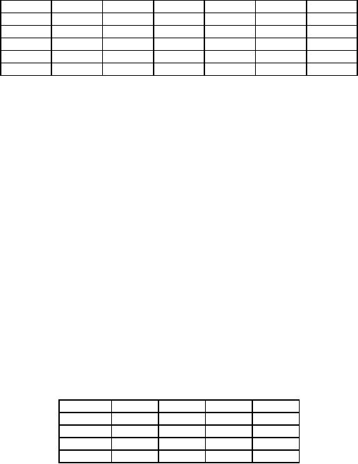
Example
2
Table
5
Destinations
Origin
P
Q
R
Supply
A
5
7
8
70
B
4
4
6
30
C
6
7
7
50
Demand
65
42
43
150
In
table 5 supply level, demands at
various destinations, and
the unit cost of
transportation are given.
Use NWC
rule
to find the initial
solution.
Solution:
The
solution obtained by the North
West Corner Rule is a basic
feasible solution. In this
method we do
not
consider the unit cost of
transportation. Hence the solution
obtained may not be an optimal
solution. But this
will
serve as an initial solution,
which can be improved.
168
Operations
Research (MTH601)
169
We
give below the procedure for
the solution of the above
problem by NWC rule.
The
North West Corner cell
(AP) is chosen for allocation.
The origin A has 70 items
and the
destination
P requires only 65 items.
Hence it is enough to allot 65 items
from A to P. The origin A
which is
alive
with 5 more items can
supply to the destination to
the right is alive with 5
more items can supply to
the
destination
to the right of P namely Q whose
requirement is 42. So, we
supply 5 items to Q thereby
the origin A
is
exhausted. Q requires 37 items
more. Now consider the
origin B that has 30 items
to spare. We allot 30
items
to
the cell (BQ) so that
the origin B is exhausted.
Then move to origin C and
supply 7 more items to
the
destination
Q. Now the requirement of
the destination Q is complete
and C is left with 43 items
and the same
can
be alloted to the destination R.
Now the origin C is emptied
and the requirement at the
destination R is also
complete.
This completes the initial solution to
the problem.
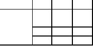
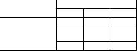
The
above calculations are
performed conveniently in a table 6 as
shown below:
Table
6
Destinations
Origin
P
Q
R
A
65
5
70
65
0
B
30
30
0
C
7
43
50
7
43
0
65
42
43
0
37
0
0
The
total cost of transportation by this
method will be
65
×
5
+
5
×
7
+
30
×
4
+
7
×
7
+
43
×
7
=
Rs.
830.
As
the solution obtained by the
North West Corner Rule may
not be expected to be particularly close
to
the
optimal solution, we have to explore a
promising initial basic feasible
solution, so that we can
teach the
optimal
solution to the problem with
minimum number of
iterations.
169
Operations
Research (MTH601)
170
Least
Cost Method
STEP
1:
Determine the least cost
among all the rows of the
transportation table.
STEP
2:Identify
the row and allocate
the maximum feasible
quantity in the cell
corresponding to the least
cost
in
the row. Then eliminate that
row (column) when an allocation is
made.
STEP
3: Repeat
steps 1 and 2 for the
reduced transportation table
until all the available
quantities are
distributed
to the required places. If
the minimum cost is not
unique, the tie can be
broken arbitrarily.
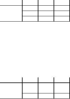
To
illustrate, consider the example
repeated in table 7
Table
7
Destination
Origin
P
Q
R
Supply
A
5
7
8
70
B
4
4
6
30
0
C
6
7
7
50
Demand
65
42
43
55
We
examine the rows A, B and C, 4 is
the least cost element in
the cell (B,P) and (B, Q)
and the tie can be
broken
arbitrarily. Select (B, P).
The origin B can supply 30
items to P and thus origin B
is exhausted. P still
requires
35 more units. Hence,
deleting the row B, we have
the reduced matrix as in the
table 8
Table
8
Destination
Origin
P
Q
R
Supply
35
A
5
7
8
70
35
C
6
7
7
50
Demand
35
42
43
0
In
the reduced matrix (table 8)
we observe that 5 is the
least element in the cell
(A, P) and examine the
supply at
A
and demand at P. The
destination P requires 35 items
and this requirement is
satisfied from A so that
the
column
P is deleted next. So we have
the reduce matrix as in
table 9
170
Operations
Research (MTH601)
171
Table
9
Destination
Origin
Q
R
Supply
35
A
7
8
35
0
C
7
7
50
Demand
42
43
7
In
the reduced matrix (table 9)
we choose 7 as least element
corresponding to the cell
(A. Q). We
supply
35 units from A to Q so have
the reduced matrix in
table10.
Table
10
Destination
Origin
Q
R
Supply
7
43
A
7
8
50
0
Demand
7
43
0
0
Now,
only one row is left
behind. Hence, we allow 7
items from C to Q and 43
items C to R.
We
now have the allotment as
per the least cost
method as shown in the table
11
Table
11
Destination
Origin
P
Q
R
Supply
A
35
35
70
B
30
30
C
7
43
50
Demand
65
42
43
The
cost of the allocation by the
least cost method is 35 x 5 + 35 x 7 + 30
x 4 + 7 x 7 + 43 x 7 = Rs. 890
Vogel's
Approximation Method
(VAM)
This
method is based on the
'difference' associated with
each row and column in the
matrix giving unit
cost
of transportation cij. This
'difference' is defined as the arithmetic
difference between the
smallest and next
to
the smallest element in that
row or column. This difference in a
row or column indicates the
minimum unit
171
Operations
Research (MTH601)
172
penalty
incurred in failing to make an allocation
to the smallest cost cell in
that row or column. This
difference
also provides a measure of
proper priorities for making allocations
to the respective rows and
column.
In
other words, if we take a
row, we have to allocate to
the cell having the
least cost and if we fail to
do so, extra
cost
will be incurred for a wrong
choice, which is called
penalty. The minimum penalty
is given by this
difference.
So, the procedure repeatedly
makes the maximum feasible
allocation in the smallest cost
cell of the
remaining
row or column, with the
largest penalty. Once an allocation is
fully made in a row or column,
the
particular
row or column is eliminated. Hence and
allocation already made cannot be
changed. Then we have
a
reduced
matrix. Repeat the same
procedure of finding penalty of
all rows and columns in the
reduced matrix,
choosing
the highest penalty in a row
or column and allotting as much as
possible in the least cost
cell in that
row
or column. Thus we eliminate another
fully allocated row or column,
resulting in further reducing
the size
of
the matrix. We repeat till
all supply and demand
are exhausted.
A
summary of the steps involved in Vogel's
Approximation Method is given
below:
STEP
1: Represent
the transportation problem in
the standard tabular
form.
STEP
2: Select
the smallest element in each
row and the next to the
smallest element in that
row. Find the
difference.
This is the penalty written on
the right hand side of each
row. Repeat the same
for each column. The
penalty
is written below each
column.
STEP
3:
Select the row or column
with largest penalty. If
there is a tie, the same
can be broken
arbitrarily.
STEP
4:
Allocate the maximum
feasible amount to the
smallest cost cell in that
row or column.
STEP
5:
Allocate zero else where in
the row or column where the
supply or demand is
exhausted.
STEP
6:
Remove all fully allocated
rows or columns from further
consideration. Then proceed
with the
remaining
reduced matrix till no rows or
columns remain.
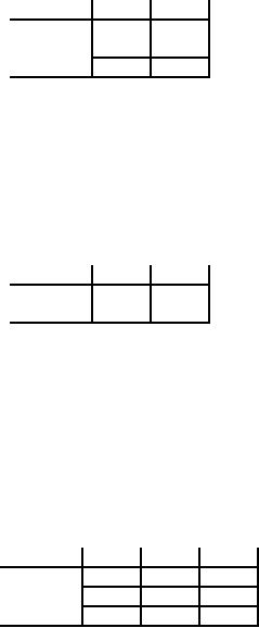
Let
us apply Vogel's Approximation Method to
the above example as given
below in table12
Table
12
Origin
Destination
Supply
Row
difference
P
Q
R
A
5
7
8
70
(2)
30
6
30
0
(0)
B
4
4
C
6
7
7
50
(1)
Demand
65
42
43
12
Column
difference (1)
(3)
(1)
Largest
Penalty
The
difference between the
smallest and next to the
smallest element in each row
and in each column is
calculated.
This is indicated in the
parenthesis. We choose the
maximum from among the
differences. The
first
individual
allocation will be to the smallest
cost of a row or column with
the largest difference. So we
select the
column
Q
(penalty
= 3) for the first
individual allocation, and
allocate to (B,
Q)
as much as we can, since
this
cell
has the least cost location.
Thus 30 units from B are
allocated to Q.
This exhausts the supply
from B.
However,
there is still a demand of 12
units from Q.
The allocations to other
cells in that column are 0,
as
indicated.
The next step is to write
down the reduced matrix
(as in table 13) eliminating
row B
(as
it is
exhausted).
172
Operations
Research (MTH601)
173
Table
13
Origin
Destination
Supply
Row
difference
P
Q
R
65
7
8
70
5
(2)
A
5
C
6
7
7
50
(1)
Demand
65
12
43
0
Column
difference (1)
(0)
(1)
From
the table 13, (2) is
the largest unit difference
corresponding to the row
A.
This leads to an allocation in the
corresponding
minimum cost location in row
A,
namely cell (A,
P).
The maximum possible allocation is
only 65
as
required by P
from
A
and
allocation of 0 to others in the row
A.
Column P
is
thus deleted and the
reduced
matrix
is given in table 14.
Maximum
difference is 1 in row A
and
in column C.
Select arbitrarily A
and
allot the least cost
cell (A,
Q)
5
units.
Delete row A.
Now,
we have only one row
C
and
two columns Q
and
R
(Table
15) indicating that all the
available amount
from
C
has
to be moved to Q
and
R
as
per their requirements.
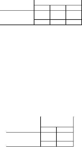
Hence we have the table
15
Table
14
Origin
Destination
Supply
Row
difference
P
R
5
8
5
0
(1)
A
7
C
7
7
50
Demand
12
43
7
Column
difference
(0)
(1)
173
Operations
Research (MTH601)
174
Table
15
Destination
Supply
Origin
Q
R
7
43
50
0
C
7
7
7
43
0
0
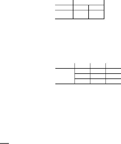
Table
16
Destination
Origin
P
Q
R
Supply
A
65
5
70
B
30
30
C
7
43
50
Demand
65
42
43
We
obtain as our basic feasible
solution by re-tracking various positive
allocations in successive
stages.
We
have the solution by Vogel's
Approximation Method as shown in the
table 16
The
cost of allocation by Vogel's Approximation Method
will be
65
×
5
+
5
×
7
+
30
×
4
+
7
×
7
+
43
×
7
=
325
+
35
+
120
+
49
+
301
=
Rs.
830.
Note:
Cost
of allocation for the same
problem with three
methods:
NWC
method - Rs. 830/-
Least
cost method -
Rs.890/-
Vogel's
Approximation Method - Rs.
830/-
Generally
VAM gives a better initial
solution.
174
Operations
Research (MTH601)
175
REVIEW
QUESTIONS
1.
What
do you mean by transportation
problem?
2.
What
do you mean by feasible solution
and basic feasible solution of
transportation problem?
3.
Describe
Transportation problem. Give a method of
finding an initial feasible
solution.
4.
Explain
in brief with examples.
(i)
North West Corner
rule.
(ii)
Vogel's Approximation Method.
5.
Explain
the classical transportation
problem and write down
its mathematical formulation and
show
that
it is a particular case of a linear
programming problem.
6.
A
petroleum company has three
major oil fields and five
oil refineries. The shipping
costs from the
fields
to the refineries, fields are as
shown in the table.
Refinery
Capacity
Production
Refinery
Barrels
per day
Field
Barrels
per day
A
10,000
1
20,000
B
13,000
2
25,000
C
13,000
3
30,000
D
16,000
E
18,000
Cost
per Barrel (Rs.)
Field
A
B
C
D
E
1
400
300
330
380
360
2
350
350
380
320
350
3
370
300
400
350
340
Determine
the optimum scheme using
the North West Corner
Rule.
Determine
the optimum scheme using
the Least Cost
Method.
Determine
the optimum scheme using
Vogel's Approximation Method.
Compare
the computations
175
Table of Contents:
- Introduction:OR APPROACH TO PROBLEM SOLVING, Observation
- Introduction:Model Solution, Implementation of Results
- Introduction:USES OF OPERATIONS RESEARCH, Marketing, Personnel
- PERT / CPM:CONCEPT OF NETWORK, RULES FOR CONSTRUCTION OF NETWORK
- PERT / CPM:DUMMY ACTIVITIES, TO FIND THE CRITICAL PATH
- PERT / CPM:ALGORITHM FOR CRITICAL PATH, Free Slack
- PERT / CPM:Expected length of a critical path, Expected time and Critical path
- PERT / CPM:Expected time and Critical path
- PERT / CPM:RESOURCE SCHEDULING IN NETWORK
- PERT / CPM:Exercises
- Inventory Control:INVENTORY COSTS, INVENTORY MODELS (E.O.Q. MODELS)
- Inventory Control:Purchasing model with shortages
- Inventory Control:Manufacturing model with no shortages
- Inventory Control:Manufacturing model with shortages
- Inventory Control:ORDER QUANTITY WITH PRICE-BREAK
- Inventory Control:SOME DEFINITIONS, Computation of Safety Stock
- Linear Programming:Formulation of the Linear Programming Problem
- Linear Programming:Formulation of the Linear Programming Problem, Decision Variables
- Linear Programming:Model Constraints, Ingredients Mixing
- Linear Programming:VITAMIN CONTRIBUTION, Decision Variables
- Linear Programming:LINEAR PROGRAMMING PROBLEM
- Linear Programming:LIMITATIONS OF LINEAR PROGRAMMING
- Linear Programming:SOLUTION TO LINEAR PROGRAMMING PROBLEMS
- Linear Programming:SIMPLEX METHOD, Simplex Procedure
- Linear Programming:PRESENTATION IN TABULAR FORM - (SIMPLEX TABLE)
- Linear Programming:ARTIFICIAL VARIABLE TECHNIQUE
- Linear Programming:The Two Phase Method, First Iteration
- Linear Programming:VARIANTS OF THE SIMPLEX METHOD
- Linear Programming:Tie for the Leaving Basic Variable (Degeneracy)
- Linear Programming:Multiple or Alternative optimal Solutions
- Transportation Problems:TRANSPORTATION MODEL, Distribution centers
- Transportation Problems:FINDING AN INITIAL BASIC FEASIBLE SOLUTION
- Transportation Problems:MOVING TOWARDS OPTIMALITY
- Transportation Problems:DEGENERACY, Destination
- Transportation Problems:REVIEW QUESTIONS
- Assignment Problems:MATHEMATICAL FORMULATION OF THE PROBLEM
- Assignment Problems:SOLUTION OF AN ASSIGNMENT PROBLEM
- Queuing Theory:DEFINITION OF TERMS IN QUEUEING MODEL
- Queuing Theory:SINGLE-CHANNEL INFINITE-POPULATION MODEL
- Replacement Models:REPLACEMENT OF ITEMS WITH GRADUAL DETERIORATION
- Replacement Models:ITEMS DETERIORATING WITH TIME VALUE OF MONEY
- Dynamic Programming:FEATURES CHARECTERIZING DYNAMIC PROGRAMMING PROBLEMS
- Dynamic Programming:Analysis of the Result, One Stage Problem
- Miscellaneous:SEQUENCING, PROCESSING n JOBS THROUGH TWO MACHINES
- Miscellaneous:METHODS OF INTEGER PROGRAMMING SOLUTION