 |
Replacement Models:REPLACEMENT OF ITEMS WITH GRADUAL DETERIORATION |
| << Queuing Theory:SINGLE-CHANNEL INFINITE-POPULATION MODEL |
| Replacement Models:ITEMS DETERIORATING WITH TIME VALUE OF MONEY >> |
Operations
Research (MTH601)
245
WHY
REPLACEMENT?
If
any equipment or machine is
used for a long period of time,
due to wear and tear,
the item tends to
worsen.
A remedial action to bring the
item or equipment to the
original level is desired. Then
the need for
replacement
becomes necessary. This need
may be caused by a loss of
efficiency in a situation leading
to
economic
decline. By efflux of time
the parts of an item are
being worn out and
the cost of maintenance
and
operation
is bound to increase year
after year. The resale
value of the item goes on
diminishing with the
passage
of
time. The depreciation of the
original equipment is a factor, which is
responsible not to favour
replacement
because
the capital is being spread
over a long time leading to a
lower average cost. Thus
there exists an
economic
trade-off between increasing
and decreasing cost
functions. We strike a balance
between the two
opposing
costs with the aim of
obtaining a minimum cost.
The problem of replacement is to
determine the
appropriate
time at which a remedial
action should be taken which
minimizes some measure of
effectiveness.
Another
factor namely technical and
/ or economic obsolescence may
force us for
replacement.
In
this segment we deal with
the replacement of capital
equipment that deteriorates
with time, group
replacement
and staffing problems.
REPLACEMENT
OF ITEMS WITH GRADUAL
DETERIORATION
As
mentioned earlier the
equipments, machineries and
vehicles undergo wear and
tear with the
passage
of
time. The cost of operation
and the maintenance are
bound to increase year by
year. A stage may be
reached
that
the maintenance cost amounts
prohibitively large that it is
better and economical to
replace the equipment
with
a new one. We also take into
account the salvage value of
the items in assessing the
appropriate or
opportune
time to replace the item. We
assume that the details
regarding the costs of
operation, maintenance
and
the
salvage value of the item
are already known. The
problem can be analysed
first without change in the
value
of
the money and later
with the value
included.
If
the interest rate for
the money is zero the
comparison can be made on an
average cost basis. The
total
cost
of the capital in owning the
item and operating is
accumulated for n
years
and this total is divided by
n.
Since
we have discrete values for
the costs for various
years, an analysis is done
using the tabular
method,
which is simple one to use
discontinuous data. There
are also the classical
optimization techniques
using
finite difference methods
for discrete parameters and
using the differential calculus
for continuous data.
Now
we take an example in which an
automobile fleet owner has the
following direct operation
cost
(Petrol
and oil) and increased
maintenance cost (repairs,
replacement of parts etc).
The initial cost of the
vehicle
is
Rs. 70, 000. The
operation cost, the
maintenance cost and the
resale price are all
given in table 1 for
five
years.
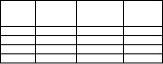
Table
1
Year
of
Annual
Annual
Resale
service
operating
maintenance
value
cost
(Rs.)
cost
(Rs.)
(Rs.)
1
10000
6000
40000
2
15000
8000
20000
3
20000
12000
15000
4
26000
16000
10000
245
Operations
Research (MTH601)
246
5
32000
20000
10000
246
Operations
Research (MTH601)
247
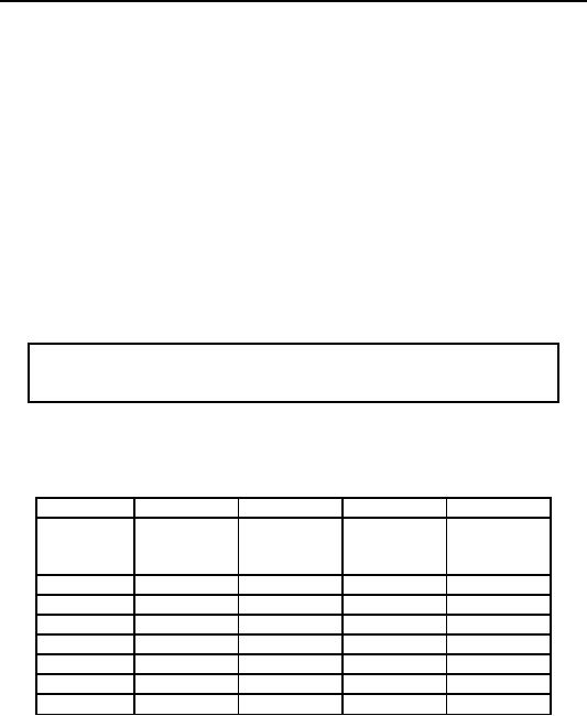
Table
2
Costs
in `000 Rupees
1
2
3
4
5
6
7
8
Capital
Total Average
Cumulative
Annual
Total
Annual
At
annual
Running
cost
cost
maintenance
running
operating
the
(Rs.)
cost
cost
(Rs.)
(Rs.)
cost
(Rs.)
cost
cost
end
(5+6)
(Rs.)
(2+3)
(Rs.)
of
(7/n)
(Rs.)
year
n
1
10
6
16
16
30
46
46.00
2
15
8
23
39
50
89
44.50
3
20
12
32
71
55
126
42.00
4
26
16
42
113
60
173
43.52
5
32
20
52
165
60
225
45.00
Table
2 gives the details of the
analysis to find the
appropriate time to replace
the vehicle. The
cumulative
running cost and capital
(Value - Resale value)
required for various years
are tabulated and
the
average
annual cost is calculated.
The corresponding year at
which this average annual
cost is minimum is
chosen
to be the opportune time of
replacement.
It
is evident from the last
column of table 2 that the
average annual cost is least
at the end of three
years.
(equal to 42,000). Hence
this is the best time to
purchase a new vehicle.
Example
A
mill owner finds from his
past records the costs of
running a machine whose
purchase price is Rs.
6000
are as given below.
Year
1
2
3
4
5
6
7
Running
cost (Rs.)
1000
1200
1400
1800
2300
2800
3400
Resale
value (Rs.)
3000
1500
750
375
200
200
200
Determine
at what age is a replacement
due?
We
prepare the following table
3 to find the
solution.
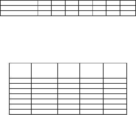
Solution:
1
2
3
4
5
At
the end
Cumulative
Capital
cost
Total
cost
Average
of
year n
running
cost
(Rs.)
(2
+ 3) (Rs.)
annual
cost
(Rs.)
(Rs.)
1
1000
3000
4000
4000
2
2200
4500
6700
3350
3
3600
5250
8850
2950
4
5400
5625
11025
2756
5
7700
5800
13500
2700
6
10500
5800
16300
2717
7
13900
5800
19700
2814
From
the above 3 we conclude that
the machine should be
replaced at the end of the
fifth year,
indicated
by the least average annual
cost (Rs. 2700) in the
last column.
247
Operations
Research (MTH601)
248
The
mill owner in the previous
problem has now three
machines, two of which are
two
Example
years
old and the third one year
old. He is considering a new type of
machine with 50% more
capacity than one
of
the old ones at a unit
price of Rs. 8000. He
estimates the running costs
and resale price for
the new machine
will
be as follows.
Year
1
2
3
4
5
6
7
Running
cost (Rs.)
1200
1500
1800
2400
3100
4000
5000
Resale
Price (Rs.)
4000
2000
1000
500
300
300
300
Assuming
that the loss of flexibility
due to fewer machines is of no
importance, and that he
will
continue
to have sufficient work for
three of the old machines,
what should his policy
be?
As
in the previous problem we
prepare a table 4 to find
the average annual cost of
the new
Solution:
type
of machine.
Table
4
At
the
Cumulative
Capital
Total
cost
Average
end
of
running
cost
(Rs.)
(Rs.)
annual
year
cost
(Rs.)
cost
(Rs.)
1
1200
4000
5200
5200
2
2700
6000
8700
4350
3
4500
7000
11500
3833
4
6900
7500
14400
3600
5
10000
7700
17700
3540
6
14000
7700
21700
3617
7
19000
7700
26700
3814
From
the above table 4 we observe
that the average annual
cost is least at the end of
five years and it
would
be Rs. 3540 per machine.
But the new machine can
handle 50% more capacity
than the old one. So
in
terms
of the old, the new machine's
annual cost is only Rs.
(3540) (2/3) = Rs. 2360.
This amount is less than
the
average
annual cost for the old
machine, which is Rs. 2700.
If we replace the old
machine with the new one, it
is
enough
to have two new machines in
place of with the new one;
it is enough to have two new
machines in place
of
three old machines. On
comparing the cost of 2 new
machines (Rs. 7080) with
that for 3 old machines
(Rs
8100),
it is clear that the policy
should be that the old
machines have to be replaced
with the new one. Still
we
have
to decide about the time
when to purchase the new
machines.
The
new machines will be purchased
when the cost for
the next year of running the
three old machines
exceeds
the average annual cost
for two new types of
machines. Examining the
table 3 pertaining to the
previous
problem,
we find, the total yearly cost of
one small machine from
the column 4. The successive
difference will
give
the cost of running a
machine for a particular
year. For example, the total
cost for 1 year is Rs.
4000. The
total
cost for 2 years is Rs.
6700. The difference of Rs.
2700 will be accounted as
the cost of running a
small
machine
during the second year.
Similarly we have Rs. 2150,
Rs. 2175, Rs. 2475
and Rs. 2800 as the
cost of
running
the old machine in the third, fourth,
fifth and sixth year
respectively.
Now,
with this information we calculate
the total costs next year
for the two smaller
machines, which
are
two years old (entering the
third year of service) and
one smaller machine aged
one year (and hence
entering
second
year of service), which will
be
2
x 2150 + 2700 = Rs.
7000
248
Operations
Research (MTH601)
249
This
is less than the average
annual cost of two new
machines, which is Rs. 7080.
So the policy is
not
to replace right now. If we
wait for the subsequent
years, the total cost of
running the old machines
will be
Rs.
6500, Rs. 7125 and
Rs. 8025 etc., for
years 2, 3 and 4 etc. This
indicates that the cost of
running the old
machine
exceeds the average annual
cost (Rs. 7000) of the
two new machines after 2
years from now. Hence
the
best
time to purchase the new
type machine will be after 2
years from now.
249
Table of Contents:
- Introduction:OR APPROACH TO PROBLEM SOLVING, Observation
- Introduction:Model Solution, Implementation of Results
- Introduction:USES OF OPERATIONS RESEARCH, Marketing, Personnel
- PERT / CPM:CONCEPT OF NETWORK, RULES FOR CONSTRUCTION OF NETWORK
- PERT / CPM:DUMMY ACTIVITIES, TO FIND THE CRITICAL PATH
- PERT / CPM:ALGORITHM FOR CRITICAL PATH, Free Slack
- PERT / CPM:Expected length of a critical path, Expected time and Critical path
- PERT / CPM:Expected time and Critical path
- PERT / CPM:RESOURCE SCHEDULING IN NETWORK
- PERT / CPM:Exercises
- Inventory Control:INVENTORY COSTS, INVENTORY MODELS (E.O.Q. MODELS)
- Inventory Control:Purchasing model with shortages
- Inventory Control:Manufacturing model with no shortages
- Inventory Control:Manufacturing model with shortages
- Inventory Control:ORDER QUANTITY WITH PRICE-BREAK
- Inventory Control:SOME DEFINITIONS, Computation of Safety Stock
- Linear Programming:Formulation of the Linear Programming Problem
- Linear Programming:Formulation of the Linear Programming Problem, Decision Variables
- Linear Programming:Model Constraints, Ingredients Mixing
- Linear Programming:VITAMIN CONTRIBUTION, Decision Variables
- Linear Programming:LINEAR PROGRAMMING PROBLEM
- Linear Programming:LIMITATIONS OF LINEAR PROGRAMMING
- Linear Programming:SOLUTION TO LINEAR PROGRAMMING PROBLEMS
- Linear Programming:SIMPLEX METHOD, Simplex Procedure
- Linear Programming:PRESENTATION IN TABULAR FORM - (SIMPLEX TABLE)
- Linear Programming:ARTIFICIAL VARIABLE TECHNIQUE
- Linear Programming:The Two Phase Method, First Iteration
- Linear Programming:VARIANTS OF THE SIMPLEX METHOD
- Linear Programming:Tie for the Leaving Basic Variable (Degeneracy)
- Linear Programming:Multiple or Alternative optimal Solutions
- Transportation Problems:TRANSPORTATION MODEL, Distribution centers
- Transportation Problems:FINDING AN INITIAL BASIC FEASIBLE SOLUTION
- Transportation Problems:MOVING TOWARDS OPTIMALITY
- Transportation Problems:DEGENERACY, Destination
- Transportation Problems:REVIEW QUESTIONS
- Assignment Problems:MATHEMATICAL FORMULATION OF THE PROBLEM
- Assignment Problems:SOLUTION OF AN ASSIGNMENT PROBLEM
- Queuing Theory:DEFINITION OF TERMS IN QUEUEING MODEL
- Queuing Theory:SINGLE-CHANNEL INFINITE-POPULATION MODEL
- Replacement Models:REPLACEMENT OF ITEMS WITH GRADUAL DETERIORATION
- Replacement Models:ITEMS DETERIORATING WITH TIME VALUE OF MONEY
- Dynamic Programming:FEATURES CHARECTERIZING DYNAMIC PROGRAMMING PROBLEMS
- Dynamic Programming:Analysis of the Result, One Stage Problem
- Miscellaneous:SEQUENCING, PROCESSING n JOBS THROUGH TWO MACHINES
- Miscellaneous:METHODS OF INTEGER PROGRAMMING SOLUTION