Portfolio and Diversification, Portfolio and Variance, Risk–Systematic & Unsystematic, Beta – Measure of systematic risk, Aggressive & defensive stocks

<< Risk and Uncertainty, Measuring risk, Variability of return–Historical Return, Variance of return, Standard Deviation

Security Market Line, Capital Asset Pricing Model – CAPM Calculating Over, Under valued stocks >>

Corporate Finance FIN 622

Lesson 16

PORTFOLIO & DIVERSIFICATION

The following topics will be discussed in this lecture.

Portfolio and Diversification

Portfolio and Variance

Risk Systematic & Unsystematic

Beta Measure of systematic risk

Aggressive & defensive stocks

Modern Portfolio Theory (MPT) proposes how rational investors will use diversification to optimize their

portfolios, and how an asset should be priced given its risk relative to the market as a whole. The basic

concepts of the theory are Mark with diversification, the efficient frontier, capital asset pricing model and

beta coefficient, the Capital Market Line and the Securities Market Line.

MPT models the return of an asset as a random variable and a portfolio as a weighted combination of

assets; the return of a portfolio is thus also a random variable and consequently has an expected value and a

variance. Risk in this model is identified with the standard deviation of portfolio return. Rationality is

modeled by supposing that an investor choosing between several portfolios with identical expected returns

will prefer that portfolio which minimizes risk.

Risk and Reward

The model assumes that investors are risk averse. This means that given two assets that offer the same

return, investors will prefer the less risky one. Thus, an investor will take on increased risk only if

compensated by higher expected returns. Conversely, an investor who wants higher returns must accept

more risk. The exact trade-off will differ by investor. The implication is that a rational investor will not

invest in a portfolio if a second portfolio exists with a more favorable risk-return profile - i.e. if for that level

of risk an alternative portfolio exists which has better expected returns.

Mean and Variance

It is further assumed that investor's risk / reward preference can be described via a quadratic utility

function. The effect of this assumption is that only the expected return and the volatility (i.e. mean return

and standard deviation) matter to the investor. The investor is indifferent to other characteristics of the

distribution of returns, such as its skew. Note that the theory uses a historical parameter, volatility, as a

proxy for risk while return is an expectation on the future.

Under the model:

· Portfolio return is the component-weighted return (the mean) of the constituent assets. Return

changes linearly with component weightings, wi.

· Portfolio volatility is a function of the correlation of the component assets. The change in volatility

is non-linear as the weighting of the component assets changes.

Diversification

An investor can reduce portfolio risk simply by holding instruments which are not perfectly correlated. In

other words, investors can reduce their exposure to individual asset risk by holding a diversified portfolio of

assets. Diversification will allow for the same portfolio return with reduced risk. For diversification to work

the component assets must not be perfectly correlated, i.e. correlation coefficient not equal to 1.

Capital Allocation Line

The Capital Allocation Line (CAL) is the line that connects all portfolios that can be formed using a risky

asset and a risk-less asset. It can be proven that it is a straight line and that it has the following equation.

In this formula P is the risky portfolio, F is the risk-less portfolio and C is a combination of portfolios P

and F.

The Efficient Frontier

Every possible asset combination can be plotted in risk-return space, and the collection of all such possible

portfolios defines a region in this space. The line along the upper edge of this region is known as the

efficient frontier (sometimes "the Mark witz"). Combinations along this line represent portfolios for which

there is lowest risk for a given level of return. Conversely, for a given amount of risk, the portfolio lying on

the efficient frontier represents the combination offering the best possible return. Mathematically the

Corporate Finance FIN 622

Efficient Frontier is the intersection of the Set of Portfolios with Minimum Variance and the Set of

Portfolios with Maximum Return.

The efficient frontier will be concave this is because the risk-return characteristics of a portfolio change in

a non-linear fashion as its component weightings are changed. (As described above, portfolio risk is a

function of the correlation of the component assets, and thus changes in a non-linear fashion as the

weighting of component assets changes.)

The region above the frontier is unachievable by holding risky assets alone. No portfolios can be

constructed corresponding to the points in this region. Points below the frontier are suboptimal. A rational

investor will hold a portfolio only on the frontier.

The Risk-Free Asset

The risk-free asset is the (hypothetical) asset which pays a risk-free rate - it is usually provied by an

investment in short-dated Government bonds. The risk-free asset has zero variance in returns (hence is

risk-free); it is also uncorrelated with any other asset (by definition: since its variance is zero). As a result,

when it is combined with any other asset, or portfolio of assets, the change in return and also in risk is

linear.

Because both risk and return change linearly as the risk-free asset is introduced into a portfolio, this

combination will plot a straight line in risk return space. The line starts at 100% in cash and weight of the

risky portfolio = 0 (i.e. intercepting the return axis at the risk-free rate) and goes through the portfolio in

question where cash holding = 0 and portfolio weight = 1.

Portfolio Leverage

An investor can add leverage to the portfolio by holding the risk-free asset. The addition of the risk-free

asset allows for a position in the region above the efficient frontier. Thus, by combining a risk-free asset

with risky assets, it is possible to construct portfolios whose risk-return profiles are superior to those on the

efficient frontier.

· An investor holding a portfolio of risky assets, with a holding in cash, has a positive risk-free

weighting (a de-leveraged portfolio). The return and standard deviation will be lower than the

portfolio alone, but since the efficient frontier is convex, this combination will sit above the

efficient frontier i.e. offering a higher return for the same risk as the point below it on the

frontier.

· The investor who borrows money to fund his/her purchase of the risky assets has a negative risk-

free weighting -i.e. a leveraged portfolio. Here the return is geared to the risky portfolio. This

combination will again offer a return superior to those on the frontier.

The Market Portfolio

The efficient frontier is a collection of portfolios, each one optimal for a given amount of risk. A quantity

known as the Sharp ratio represents a measure of the amount of additional return (above the risk-free rate)

a portfolio provides compared to the risk it carries. The portfolio on the efficient frontier with the highest

Sharpe Ratio is known as the market portfolio, or sometimes the super-efficient portfolio. This portfolio

has the property that any combination of it and the risk-free asset will produce a return that is above the

efficient frontier - offering a larger return for a given amount of risk than a portfolio of risky assets on the

frontier would.

Capital Market Line

When the market portfolio is combined with the risk-free asset, the result is the Capital Market Line. All

points along the CML have superior risk-return profiles to any portfolio on the efficient frontier. (A

position with zero cash weighting is on the efficient frontier - the market portfolio.)

The CML is illustrated above, with return μp on the y axis, and risk σp on the x axis.

One can prove that the CML is the optimal CAL and that its equation is:

Asset Pricing

A rational investor would not invest in an asset which does not improve the risk-return characteristics of his

existing portfolio. Since a rational investor would hold the market portfolio, the asset in question will be

added to the market portfolio. MPT derives the required return for a correctly priced asset in this context.

Corporate Finance FIN 622

Systematic Risk and Specific Risk

Specific risk is the risk associated with individual assets - within a portfolio these risks can be reduced

through diversification (specific risks "cancel out"). Systematic risk, or market risk, refers to the risk

common to all securities - except for selling short as noted below, systematic risk cannot be diversified away

(within one market). Within the market portfolio, asset specific risk will be diversified away to the extent

possible. Systematic risk is therefore equated with the risk (standard deviation) of the market portfolio.

Since a security will be purchased only if it improves the risk / return characteristics of the market portfolio,

the risk of a security will be the risk it adds to the market portfolio. In this context, the volatility of the asset,

and its correlation with the market portfolio, is historically observed and is therefore a given (there are

several approaches to asset pricing that attempt to price assets by modeling the stochastic properties of the

moments of assets' returns - these are broadly referred to as conditional asset pricing models). The

(maximum) price paid for any particular asset (and hence the return it will generate) should also be

determined based on its relationship with the market portfolio.

Systematic risks within one market can be managed through a strategy of using both long and short

positions within one portfolio, creating a "market neutral" portfolio.

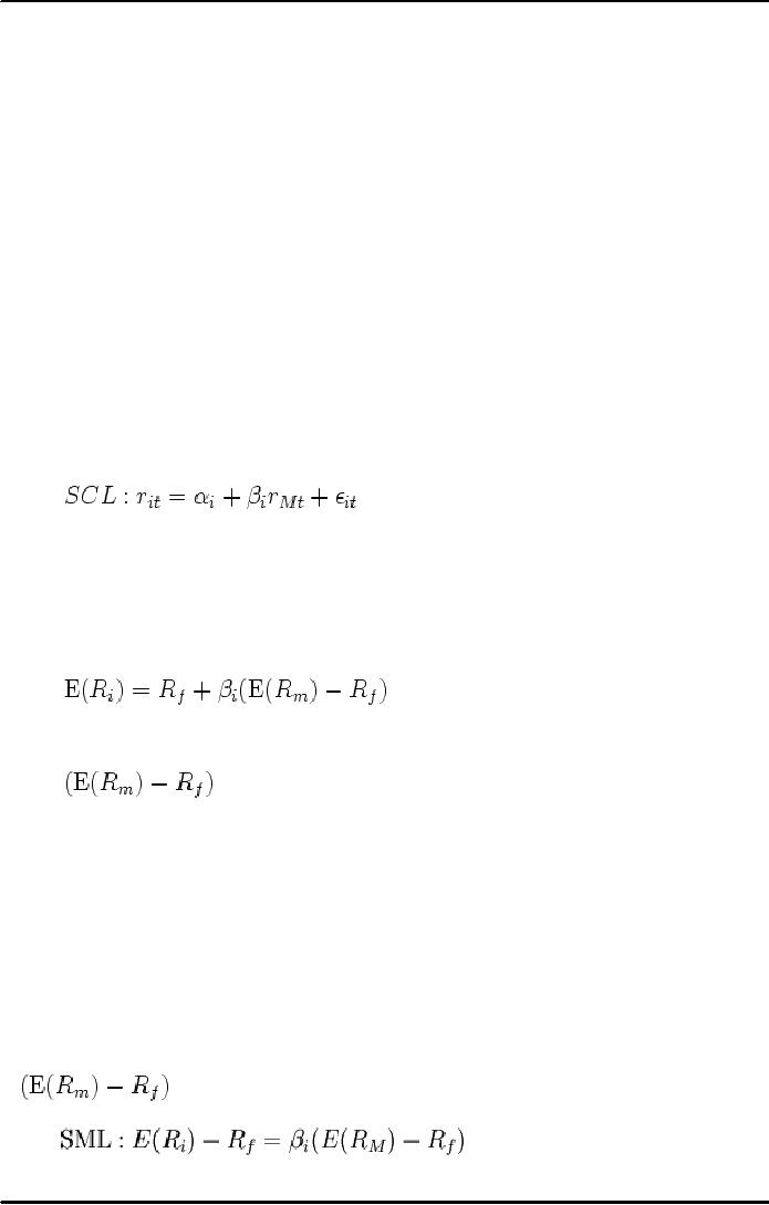
Security Characteristic Line

The Security Characteristic Line (SCL) represents the relationship between the market return (rM) and

the return of a given asset i (ri) at a given time t. In general, it is reasonable to assume that the SCL is a

straight line and can be illustrated as a statistical equation:

where αi is called the asset's alpha coefficient and βi the asset's beta coefficient.

Capital asset pricing model

The asset return depends on the amount paid for the asset today. The price paid must ensure that the

market portfolio's risk / return characteristics improve when the asset is added to it. The CAPM is a model

which derives the theoretical required return (i.e. discount rate) for an asset in a market, given the risk-free

rate available to investors and the risk of the market as a whole.

The CAPM is usually expressed:

β, Beta, is the measure of asset sensitivity to a movement in the overall market; Beta is usually

found via regression on historical data. Betas exceeding one signify more than average "risk ness";

betas below one indicate lower than average.

is the market premium, the historically observed excess return of the market

over the risk-free rate'

Once the expected return, E(ri), is calculated using CAPM, the future cash flows of the asset can be

discounted to their present value using this rate to establish the correct price for the asset. (Here again, the

theory accepts in its assumptions that a parameter based on past data can be combined with a future

expectation.)

A more risky stock will have a higher beta and will be discounted at a higher rate; less sensitive stocks will

have lower betas and be discounted at a lower rate. In theory, an asset is correctly priced when its observed

price is the same as its value calculated using the CAPM derived discount rate. If the observed price is

higher than the valuation, then the asset is overvalued; it is undervalued for a too low price.

Securities Market Line

The relationship between Beta & required return is plotted on the securities market line (SML) which shows

expected return as a function of β. The intercept is the risk-free rate available for the market, while the slope

. The Securities market line can be regarded as representing a single-factor model of

the asset price, where Beta is exposure to changes in value of the Market. The equation of the SML is thus:

Corporate Finance FIN 622

Comparison with Arbitrage Pricing Theory

The SML and CAPM are often contrasted with the Arbitrage pricing theory (APT), which holds that the

expected return of a financial asset can be modeled as a linear function of various macro-economic factors,

where sensitivity to changes in each factor is represented by a factor specific bets coefficient.

The APT is less restrictive in its assumptions: it allows for an explanatory (as opposed to statistical) model

of asset returns, and assumes that each investor will hold a unique portfolio with its own particular array of

betas, as opposed to the identical "market portfolio". Unlike the CAPM, the APT, however, does not itself

reveal the identity of its priced factors - the number and nature of these factors is likely to change over time

and between economies.

Table of Contents: