Perception:BRIGHTNESS SENSITIVITY, Wavelength sensitivity, OPTICAL ILLUSIONS

<< Tools:CONVOLUTION, FOURIER TRANSFORMS, Circularly symmetric signals

Image Sampling:Sampling aperture, Sampling for area measurements >>

...Image Processing Fundamentals

Perception

Many image processing applications are intended to produce images that are to be

viewed by human observers (as opposed to, say, automated industrial inspection.)

It is therefore important to understand the characteristics and limitations of the

human visual system--to understand the "receiver" of the 2D signals. At the outset

it is important to realize that 1) the human visual system is not well understood, 2)

no objective measure exists for judging the quality of an image that corresponds to

human assessment of image quality, and, 3) the "typical" human observer does not

exist. Nevertheless, research in perceptual psychology has provided some

important insights into the visual system. See, for example, Stockham [12].

4.1 BRIGHTNESS SENSITIVITY

There are several ways to describe the sensitivity of the human visual system. To

begin, let us assume that a homogeneous region in an image has an intensity as a

function of wavelength (color) given by I(λ). Further let us assume that I(λ) = Io, a

constant.

4.1.1 Wavelength sensitivity

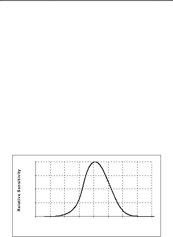
The perceived intensity as a function of λ, the spectral sensitivity, for the "typical

observer" is shown in Figure 10 [13].

1.00

0.75

0.50

0.25

0.00

350

400

450

500

550

600

650

700

750

Wavelength (nm.)

Figure 10: Spectral Sensitivity of the "typical" human observer

4.1.2 Stimulus sensitivity

If the constant intensity (brightness) Io is allowed to vary then, to a good

approximation, the visual response, R , is proportional to the logarithm of the

intensity. This is known as the WeberFechner law:

...Image Processing Fundamentals

R = log( Io )

(45)

The implications of this are easy to illustrate. Equal perceived steps in brightness,

ĆR = k, require that the physical brightness (the stimulus) increases exponentially.

This is illustrated in Figure 11ab.

A horizontal line through the top portion of Figure 11a shows a linear increase in

objective brightness (Figure 11b) but a logarithmic increase in subjective

brightness. A horizontal line through the bottom portion of Figure 11a shows an

exponential increase in objective brightness (Figure 11b) but a linear increase in

subjective brightness.

256

192

Ć I=k

128

Ć I=k·I

Sampled Postion

Figure 11a

Figure 11b

(top) Brightness step ĆI = k

Actual brightnesses plus interpolated values

(bottom) Brightness step ĆI = k·I

The Mach band effect is visible in Figure 11a. Although the physical brightness is

constant across each vertical stripe, the human observer perceives an "undershoot"

and "overshoot" in brightness at what is physically a step edge. Thus, just before

the step, we see a slight decrease in brightness compared to the true physical value.

After the step we see a slight overshoot in brightness compared to the true physical

value. The total effect is one of increased, local, perceived contrast at a step edge in

brightness.

4.2 SPATIAL F REQUENCY SENSITIVITY

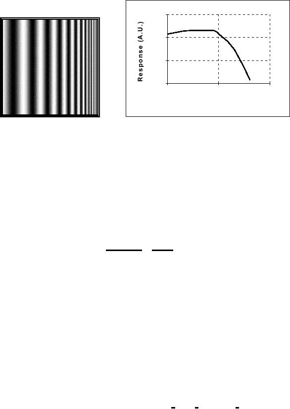
If the constant intensity (brightness) Io is replaced by a sinusoidal grating with

increasing spatial frequency (Figure 12a), it is possible to determine the spatial

frequency sensitivity. The result is shown in Figure 12b [14, 15].

...Image Processing Fundamentals

1000

100

Spatial Frequency

(cycles/degree)

Figure 12a

Figure 12b

Sinusoidal test grating

Spatial frequency sensitivity

To translate these data into common terms, consider an "ideal" computer monitor

at a viewing distance of 50 cm. The spatial frequency that will give maximum

response is at 10 cycles per degree. (See Figure 12b.) The one degree at 50 cm

translates to 50 tan(1°) = 0.87 cm on the computer screen. Thus the spatial

frequency of maximum response fmax = 10 cycles/0.87 cm = 11.46 cycles/cm at

this viewing distance. Translating this into a general formula gives:

572.9

f max =

cycles / cm

(46)

d · tan(1°)

where d = viewing distance measured in cm.

4.3 COLOR SENSITIVITY

Human color perception is an exceedingly complex topic. As such we can only

present a brief introduction here. The physical perception of color is based upon

three color pigments in the retina.

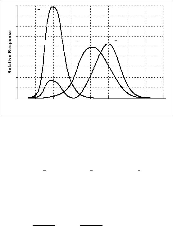
4.3.1 Standard observer

Based upon psychophysical measurements, standard curves have been adopted by

the CIE (Commission Internationale de l'Eclairage) as the sensitivity curves for the

"typical" observer for the three "pigments" x (λ ), y (λ), and z (λ ) . These are

shown in Figure 13. These are not the actual pigment absorption characteristics

found in the "standard" human retina but rather sensitivity curves derived from

actual data [10].

...Image Processing Fundamentals

z(λ )

x (λ )

y (λ )

350

400

450

500

550

600

650

700

750

Wavelength (nm.)

Figure 13: Standard observer spectral sensitivity curves.

For an arbitrary homogeneous region in an image that has an intensity as a function

of wavelength (color) given by I(λ), the three responses are called the tristimulus

values:

∞

X = ∫ I( λ )x (λ )dλ

Y = ∫ I( λ ) y (λ )dλ

Z = ∫ I (λ )z ( λ) dλ

(47)

4.3.2 CIE chromaticity coordinates

The chromaticity coordinates which describe the perceived color information are

defined as:

z = 1 - ( x + y)

(48)

X+Y+Z

X + Y +Z

The red chromaticity coordinate is given by x and the green chromaticity coordinate

by y. The tristimulus values are linear in I(λ) and thus the absolute intensity

information has been lost in the calculation of the chromaticity coordinates {x,y}.

All color distributions, I(λ), that appear to an observer as having the same color

will have the same chromaticity coordinates.

If we use a tunable source of pure color (such as a dye laser), then the intensity can

be modeled as I(λ) = δ(λ λo) with δ(·) as the impulse function. The collection of

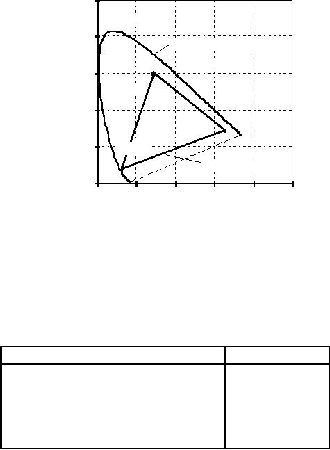
chromaticity coordinates {x,y} that will be generated by varying λo gives the CIE

chromaticity triangle as shown in Figure 14.

...Image Processing Fundamentals

1.00

520 nm.

0.80

Chromaticity Triangle

560 nm.

0.60

500 nm.

0.40

640 nm.

0.20

470 nm.

Phosphor Triangle

0.00

0.20

0.40

0.60

0.80

1.00

Figure 14: Chromaticity diagram containing the CIE chromaticity

triangle associated with pure spectral colors and the triangle associated

with CRT phosphors.

Pure spectral colors are along the boundary of the chromaticity triangle. All other

colors are inside the triangle. The chromaticity coordinates for some standard

sources are given in Table 6.

Source

Fluorescent lamp @ 4800 °K

0.35

0.37

Sun @ 6000 °K

0.32

0.33

Red Phosphor (europium yttrium vanadate)

0.68

0.32

Green Phosphor (zinc cadmium sulfide)

0.28

0.60

Blue Phosphor (zinc sulfide)

0.15

0.07

Table 6: Chromaticity coordinates for standard sources.

The description of color on the basis of chromaticity coordinates not only permits

an analysis of color but provides a synthesis technique as well. Using a mixture of

two color sources, it is possible to generate any of the colors along the line

connecting their respective chromaticity coordinates. Since we cannot have a

negative number of photons, this means the mixing coefficients must be positive.

Using three color sources such as the red, green, and blue phosphors on CRT

monitors leads to the set of colors defined by the interior of the "phosphor

triangle" shown in Figure 14.

...Image Processing Fundamentals

The formulas for converting from the tristimulus values (X,Y,Z) to the well-known

CRT colors (R ,G,B ) and back are given by:

R  1.9107 -0.5326 -0.2883  X 

G = -0.9843 1.9984 -0.0283 · Y 

(49)

  

  

 B  0.0583 - 0.1185 0.8986   Z

 

  



and

 X  0.6067 0.1736 0.2001  R

 Y  = 0.2988 0.5868 0.1143 · G

(50)

  

  

Z  0.0000 0.0661 1.1149  B

  

  

As long as the position of a desired color (X,Y,Z) is inside the phosphor triangle in

Figure 14, the values of R , G, and B as computed by eq. (49) will be positive and

can therefore be used to drive a CRT monitor.

It is incorrect to assume that a small displacement anywhere in the chromaticity

diagram (Figure 14) will produce a proportionally small change in the perceived

color. An empirically-derived chromaticity space where this property is

approximated is the (u',v') space:

u' =

v' =

-2 x + 12 y + 3

and

(51)

9u'

4v'

6u' -16 v' + 12

6u' - 16v' +12

Small changes almost anywhere in the (u',v') chromaticity space produce equally

small changes in the perceived colors.

4.4 OPTICAL ILLUSIONS

The description of the human visual system presented above is couched in standard

engineering terms. This could lead one to conclude that there is sufficient

knowledge of the human visual system to permit modeling the visual system with

standard system analysis techniques. Two simple examples of optical illusions,

shown in Figure 15, illustrate that this system approach would be a gross

oversimplification. Such models should only be used with extreme care.

Table of Contents: