Miscellaneous:SEQUENCING, PROCESSING n JOBS THROUGH TWO MACHINES

<< Dynamic Programming:Analysis of the Result, One Stage Problem

Miscellaneous:METHODS OF INTEGER PROGRAMMING SOLUTION >>

Operations Research (MTH601)

270

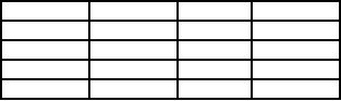
10000

20000

30000

40000

50000

Segment X: Miscellaneous

Lectures 44-45

270

Operations Research (MTH601)

271

SEQUENCING

INTRODUCTION

A series, in which a few jobs or tasks are to be performed following an order, is called

sequencing. In such a situation, the effectiveness measure (time, cost, distance etc.,) is a function of

the order or sequence of performing a series of jobs. Problems of sequencing can be classified into

two major groups.

In the first type of problem, we have n jobs to perform each of which requires processing on

some or all m different machines. If we analyze the number of sequences, it runs to (n!)m possible

sequences and only a few of them are technologically feasible, i.e., those which satisfy the constraints

on the order in which each task has to be processed through m machines.

In the second type of problem, we have a situation with a number of machines and a series

jobs to perform. Once a job is finished, we have to take a decision on the next job to be started.

Practically both types of problems seem to be intrinsically difficult and now we know solutions

only for some special cases of the first type of problem. For the second type of problems, it appears

that a few empirical rules have been obtained to arrive at the solution and mathematical theory has to

be explored.

PROCESSING n JOBS THROUGH TWO MACHINES

The sequencing problem with n jobs through two machines can be solved easily. S.M.

Johnson has developed solution procedure. The problem can be stated as follows.

Only two machines are involved, A and B.

Each job is processed in the order AB.

The exact or expected processing times A1, A2, ..., An, B1, B2, ..., Bn are known.

A decision has to be arrived to find the minimum elapsed time from the start of the first job to

the completion of the last job. It has been established that the sequence that minimizes the elapsed

time are the same for both machines. The algorithm for solving the problem is as follows and due to

S.M. Johnson.

Select the smallest processing time occurring in the list, A1, ..., An, B1, ... , Bn. If there

is a tie, break the tie arbitrarily.

If the minimum processing time is Ai, do the ith job first. If it is Bj do the j-th job last.

This decision is applicable to both machines A and B.

Having selected a job to be ordered, there are now n-1, jobs left to be ordered. Apply

the steps 1 and 2 to the reduced set of processing times obtained by deleting the two

machine processing times corresponding to the job that is already assigned.

Continue in this manner until all jobs have been ordered. The resulting ordering will

minimize the elapsed time, T.

THE TRAVELLING SALESMAN PROMLEM

In this type of problem, we have to select a route by a salesman that will minimize the total

distance traveled in visiting n cities and returning to the starting point. Another example is that if n

271

Operations Research (MTH601)

272

products are to be made in some order on a continuing basis, and the set up cost for each

depends on the preceding product made, we want to find cost for each depends on the preceding

products that will minimize the total set up cost when the product Ai is followed by Aj. The set up costs

are represented in square matrix, while the leading diagonal blank, indicating no set up cost when

changing a product to itself. In traveling salesman problem, we cannot choose the element along the

diagonal and this can be avoided by filling the diagonal with infinitely large elements. Another

constraint we have to work with is that having started from a station Ai say, we do not want to go to

the same station again until we have moved to all other stations.

INTEGER PROGRAMMING

INTRODUCTION

In linear programming problem, the decision variables represent men, machines, vehicles,

number of items to be produced etc. These variables make sense only if they have integer values in

the final solution to the linear programming problem. This is the problem faced in real life practice. For

example, if we get a solution to a problem when we decide on the number of chairs and tables

produced per day in a furniture industry. As 2.53 chairs and 3.82 tables, it is meaningless because of

non-integer solution. Hence a new procedure has been developed in this direction for the case of

linear programming problems subjected to the additional restriction that the decision variables must

have integer values.

For solving this type of integer linear programming problems, the usual technique is to apply

the simplex method ignoring the integer restriction and then rounding off the non-integer values to

integers in the resulting solution. There are some pitfalls in this approach. One is that it is difficult to

see in which way the rounding off should is rounded off successfully, there is no guarantee that this

rounded-off solution will be the optimal integer solution. In fact it may be far from optimal in terms of

the value of the objective function.

This can be illustrated by the following problem.

Maximize

Z = 2x + 10y

x + 10y < 20

Subject to

and x and y are non-negative integers.

Since this problem involves only two variables, a graphical solution can be easily obtained which is

given below.

The graphical solution is used to find the optimal integer solution or optimal non-integer

solution. The optimal non-integer solution should be x = 2 and y = 9/5 with Z* = 22. If the simple

procedure is adopted, then the variable with the non-integer value y = 9/5 in rounded off in the

feasible direction to y = 1. Then the resulting integer solution is x = 2, y = 1 and Z* = 14. But this is far

from the optimal solution,

(x, y) = (0, 2) where Z* = 20

Therefore an efficient solution procedure for obtaining an optimal solution to integer

programming problems is necessary. Some progress has been made in recent years in developing

algorithms (solution procedures) for integer programming problems.

272

Table of Contents: