 |
Linear Programming:SOLUTION TO LINEAR PROGRAMMING PROBLEMS |
| << Linear Programming:LIMITATIONS OF LINEAR PROGRAMMING |
| Linear Programming:SIMPLEX METHOD, Simplex Procedure >> |
Operations
Research (MTH601)
103
SOLUTION
TO LINEAR PROGRAMMING
PROBLEMS
Having
formulated a linear programming
problem, we have to find the
solution for the same. To
find the
solution
to a linear programming model, we
have the graphical and
the algebraic methods that
can be applied
successfully.
If
the problem involves only
two decision variables,
graphical method of solution is quite
adequate. Even
when
three decision variables are
involved, a graphical solution can be
resorted to. But this
involves three-
dimensional
representation. Therefore we can
conveniently restrict the
graphical method to problems
involving two
decision
variables.
The
second method is the
algebraic procedure or simplex
method, which involves an iterative
procedure.
This
can be applied to linear
programming problems involving
two or more variables. This is
the most versatile
method
of solving linear programming models. In
this method, an initial solution is
assumed and this solution s
modified
progressively through a well-defined
iterative process until we
get the optimal solution.
The procedure is
simple
and so mechanical that it
requires time and patience
to execute it manually. However, an
electronic computer
with
the readymade programmes can
be used as a handy tool for
solving LP problems involving many
variables.
Graphical
solution to LPP
We
all know that a point can be
represented by two co-ordinates
namely and x
and
y
in
a graph. From the
origin
we have to go x
units
along x
axis
and y
units
along y-axis. If we plot two
points in a graph and join
them we
get
a segment of a straight line. A minimum
of two points is needed to a draw a
straight line. In a linear
programming
problem, the objective function
and constraints are linear, so
that we can plot the
straight lines
representing
constraints and the
objectives function.
Let
us take an algebraic equation
3x
+
5y
=15.
This is a first-degree equation in x
and y. Geometrically this
represents
a straight line. If we want to represent
the above equation geometrically, we
require a minimum of
two
points
to plot a line. Let x
=
0, we get y
=
3 and let y
=
0 we get x
=
5. Hence we have two points
A(0,
3) and B(5,
0)
and
connect them to get a
straight line
Fig
1
103
Operations
Research (MTH601)
104
We
normally come across, in
linear programming problems,
the linear constraints
having inequalities
either
'greater
than equal to' or 'less
than equal to' or strictly
'equal to'.
Consider
the inequality
3x +
5y
<
15
To
plot the feasible area
satisfying the above inequality, we
consider the equation
3x +
5y
=
15.
This
has been plotted in the
figure 1. This straight line has an
area above the line
and an area below
the
line.
To determine the appropriate
area satisfying the inequality,
3x
+
5y
<
15,
Let
us consider the origin
(x
=
0, y
=
0) as a reference point. Left hand
side for the reference point
is 3.0 + 5.0 = 0.
The
value '0' of the left
hand side, is clearly less
than 15 satisfying the constraint
and therefore the
origin
whose
co-ordinates are (0, 0) is a point to be
included in the feasible
area. The origin is below
the straight line
and
the
area A1 should also contain
the trial point namely the
origin. Hence the feasible
area satisfying the constraint
3x
+
5y
<
15 is indicated as A1 in figure 2.
Fig.
2
Next
consider the inequality
3x +
5y
>
15
To
find the feasible area
satisfying the above inequality, we take
once again the origin as a
trial point and
see
whether this has to be
included in the area. Let
x
=
0 and y
=
0, then we get the value of
the left hand side is
0
and
the right hand side is 15
and hence the area
satisfying this space inequality
3x
+
5y
>
15, should not contain
the
origin
and hence the feasible
solution space is as indicated by
A2 in figure 3.
The
constraints are linear in a
linear programming problem,
which can be plotted on a
graph. The ingenuity
of
graphical solution to a linear
programming problem depends on
fixing the proper solution
space.
Consider
the following inequality 4x
-
5y
<
20
To
get the feasible space to
satisfy the above
constraint, first we plot
the straight line 4
x
-
5y
=
20 as shown
in
figure 4. The origin, which
satisfies the constraint,
should be included in the solution
space.
104
Operations
Research (MTH601)
105
Fig.
3
Fig.
4
Hence
the area above the
straight line shows the
feasible solution space satisfying the
inequality 4x
-
5y
<
20.
The area below the
line will correspond to the
constraint 4x
-
5y
>
20.
Consider
the inequality
-4x +
5y
<
20
We
plot the straight line
-4x
+
5y
=
20 as shown in figure 5
The
origin satisfies the inequality
-4x + 5y < 20 and this
should be included in the
feasible solution space. Hence
the
area
below the straight line
should represent the
feasible solution space
Consider
the inequality
-4x -
5y
<
20
We
plot the straight line
-4x
-
5y
=
20 as shown in figure 6
Fig
5
Fig.
6
Since
the origin satisfies the
inequality -4x
-
5y
=
20 it should be included in the
feasible solution space. Hence
the
area
above the straight line
should be the solution
space.
Procedure
for Graphical Solution to
LPP
Having
explained how to fix the
feasible solution space satisfying the
constraint, we now give various
steps
involved
in arriving at a solution to a linear
programming problem.
STEP
1:Consider
all the constraints. Taking
the equality relationship, plot
all the straight lines in a
graph and get
feasible
solution space satisfying the inequality.
Usually we get a bounded solution
space.
105
Operations
Research (MTH601)
106
STEP
2:
Assign an arbitrary value for
the objective function. Plot the
straight line to represent
the objective
function,
with the arbitrary value
for Z.
STEP
3:
Move the objective line
parallel in the appropriate direction in
the solution space to maximize
and in the
opposite
direction to minimize the objective
function under consideration.
STEP
4:
In this process, the moving
objective line may meet an
extreme point (or corner point)
beyond which we
cannot
proceed as this violates the
constraints. Note the co-ordinates of
this extreme point, which
will give
maximum
or minimum value of the
objective function.
The
above steps are explained in
the following
example.
Example
Maximize
Z = 4x
+
7y
Subject
to
x
<
40, y
<
30, x
+ y <
60,
x,
y >
0
In
the above example, we have
three constraints and all of
them are 'less than
inequalities'. First step in
the
graphical
method of solution to the linear
programming problem is to represent
the constraints graphically.
Consider
the
first constraint
x
<
40
This
indicates that x
can
take a value 40 or less than
40, for all values of
y.
The equation x
=
40 is a straight
line
parallel to the y
axis
as in the figure 2.7 and the
area to the left of this
straight line is the solution
space
satisfying
the constraint x
<
40.
Fig.
7
Fig.
8
Consider
the second constraint
y
<
30. This demands that
y
can
take a value of 30 or less
than 30 for all
the
values
of x.
The equation y
=
30 is a line parallel to x-axis
and is represented in figure 8.
Similarly
consider the third constraint
x
+ y <
60. To plot the straight
line let x
=
0, then y
=
60 and let y
=
0,
then x
=
60. Therefore the two
points (0, 60) and
(60, 0) represented in figure 9 will be
connected, to get the
straight
line x
+
y
=
60. To get the solution
space satisfying x
+ y <
60, let x
=
0 and y
=
0, then the left hand
side
106
Operations
Research (MTH601)
107
reduces
to 0 which is clearly less than
60. Therefore the area
below the line including
(0, 0) represented by
the
shaded
portion in figure 9 represents the
solution space satisfying the constraint
x
+ y =
60.
Fig.
9
Consider
the non-negative constraints
for x
an
y
and
the feasible solution space is
obtained by combining
all
the constraints in one figure as
shown in figure 10.
The
shaded portion of the figure 10
represents the solution space as
feasible region. The solution
space in
figure
2.10 is a bounded figure with
five corner points
(otherwise called extreme
points) namely A,
B, C, D and
E.
The
solution space is bounded by segments of
five straight lines. The
co-ordinates of A,
B, C, D and
E
are
determined
by solving the appropriate simultaneous
constraint equations.
Thus
we have A
at
the origin, having xo-ordinates
x
=
0, y
=
0.
The
co-ordinates for B
are
x
=
0, y
=
30.
The
co-ordinates of C
are
found by solving equations:
y
=
30
x
+ y =
60
Fig
10
Fig
11
We
get the co-ordinates of
C
as
x
=
30, y
=
30.
Similarly
the co-ordinates of D
are
determined by solving equations:
107
Operations
Research (MTH601)
108
x
=
40
x
+ y =
60
The
co-ordinates of D
are
x
=
40, y
=
20
The
co-ordinates of E
are
x
=
40, y
=
0.
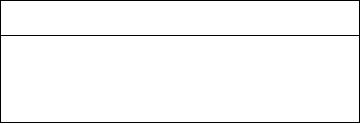
The
next step is to examine the
value of the objective function at
these points. This is done in
the table
below:
Extreme
point
Co-ordinates
Value
of
or
corner point
Z
=
4x
+
7y
A
(0,
0)
0
B
(0,
30)
210
C
(30,
30)
330*
D
(40,
20)
300
E
(40,
0)
160
From
the above table we see
that the objective function
has a maximum value of 330
at C
(30,
30). So, the
optimum
Z
denoted
by Z*
is
given by Z*
=
330 for x
=
30 and y
=
30.
Alternate
Method:
Instead
of evaluating the objective function at
all the extreme points; a
graphical optimum solution can
be
obtained
which is explained
below.
Consider
the objective function
Z
=
4x
+
7y
Assign
a convenient arbitrary value
for Z
say
Z
=
140, then
Z
=
4x
+
7y
=
140
This
is a straight line, which can be
represented in the solution space as
shown in figure 11.
Consider
Z = 4x
+
7y
=
140. If x
=
0, we get y
=
20 and if y
=
0, we get x
=
35. These two points
are connected by a
straight
line representing Z =
140.
Thus
Z
=
140 is called an iso-profit line
since for all points in
the straight line, Z
=
140. With this value
we
have
obtained the slope and
hence shape of the straight
line.
Next
step is to draw straight lines
parallel to 4x
+
7y
=
140.
108
Operations
Research (MTH601)
109
This
results in moving the
objective line with various
values in the solution space in a
proper direction
(upwards
in this example for
maximization and downwards
for minimization). In this process,
the objective line
may
cross
a corner point indicating the maximum or
minimum value.
Drawing
parallel lines we see that a
line passing through
C
(30,
30) gives the maximum
value for Z
and
value
of Z*
=
330.
Example
Minimize
Z
=
4x
+
5y
Subject
to
x
+ y >
10
2x +
5y
>
35
x,
y >
0
Solution
STEP
1 Represent
the constraints graphically
Consider
x
+ y =
10
If
x
=
0, then y
=
10
If
y
=
0, then x
=
10
Consider
2x +
5y
=
35
If
x
=
0, then y
=
7
If
y
=
0, then x
=
17.5
The
above constraints are
represented in figure 12.
STEP
2:
Mark
the solution space in the
graph satisfying all the
constraints.
Fig.
12
Choose
an arbitrary value of Z,
say 100. Then
STEP
3
Z
=
4x
+
5y
=
100
109
Operations
Research (MTH601)
110
If
x
=
0, then y
=
20
If
y
=
0, then x
=
25
Represent
Z
=
100 in the graph.
Move
down the line Z =
100 to minimize the total
cost Z.
Thus we get the minimum
value of Z
at
the point B,
which
is
the intersection of two
lines:
x
+ y =
10
2x +
5y
=
35
Solving
the two equations, we get
x
=
5, y
=
5
The
minimum value of Z
=
4 x 5 + 5 x 5 = 45,
Therefore,
Z*
=
45, x
=
5, y
=
5
RESULT:
Certain
Definitions:
1.
A
feasible solution is the value of
all points for which
all constraints are
satisfied.
2.
An
optimal solution is a feasible solution,
which maximizes or minimizes
the objective function.
These
terms can be interpreted in
terms of the graphical
representation. The feasible solution
includes all
the
points within the
permissible region (or solution
space) including the boundary
points.
110
Operations
Research (MTH601)
111
REVIEW
QUESTIONS
6.
The
standard weight of a brick is 5
kg, and it
Solve
Graphically
contains
two basic ingredients
B1 and B2.B1 costs Rs.
5/kg
and B2 costs Rs. 8/kg Strength
considerations
1.
Maximize
Z
=
3x
+
7y
dictate
that the brick contains
not more than 4 kg of
B1 and a minimum of 2 kg of
B2. Since the
demand
Subject
to
for
the product is likely to be
related to the price
of
x
+
4y
<
20
the
brick, find out graphically
the minimum cost of
2x +
y
<
30
the
brick satisfying the above
conditions.
x+y<8
and
x,
y >
0
7.
Solve
by graphical method the
following
problem.
2.
Maximize
Z = 2x + 3y
Minimize
Subject
to
-x +
2y
<
16
Z
=
5x1 + 4x2
Subject
to
4x1 + x2 > 40
x
+
y
<
24
x
+
3y
>
45
2x1 + 3x2 > 90
-4x +
10y
>
20
and
x,
y > 0
x1 > 0, x2 > 0
3.
Maximize
Z
=
3x1 + 5x2
b)
Food A
contains
20 units of vitamin x
and
40 units
Subject
to
-3x1 + 4x2 < 12
of
vitamin y
per
gram. Food B
contains
30 units of
2x1 - x2 > -2
each
of vitamins x
and
y.
The daily minimum
human
2x1 + 3x2 > 12
requirements
of vitamin x
and
y
are
900 units and
1200
units respectively. How many
grams of each
x1 < 4
type
of food should be consumed so as to
minimize
x2 > 2
the
cost, if food A
costs
60 paise per gram and
food B
x1 > 0
80
paise per gram.
4.
Maximize
Z
=
4x1 + 6x2
8.
A
company produces two types
of products
say
type A and type B. Product A
is of superior
Subject
to
x1 < 2
quality
and product B is of a lower
quality.
x2 < 4
Respective
profits for the two types of
products are
x1 + x2 > 3
Rs.
40/- and 30/-. The
data on the resource
required,
and
x1, x2 > 0
availability
of resources are given
below:
5.
What
are the four major types of
allocation
Capacity
Requirements
problems,
which could be solved using
linear
Product
A
Product
B
available
programming
technique? Briefly explain each
one of
Per
month
them
with an example.
Raw
materials
120
60
12000
(kg)
b)
Minimize
Z
=
4x1 + x2
Machining
time
5
8
600
(hrs/piece)
Subject
to
3x1 + 4x2 > 20
Assembly
4
3
500
-x1 - 5x2 < -15
(man-hour)
and
x1, x2 > 0
111
Table of Contents:
- Introduction:OR APPROACH TO PROBLEM SOLVING, Observation
- Introduction:Model Solution, Implementation of Results
- Introduction:USES OF OPERATIONS RESEARCH, Marketing, Personnel
- PERT / CPM:CONCEPT OF NETWORK, RULES FOR CONSTRUCTION OF NETWORK
- PERT / CPM:DUMMY ACTIVITIES, TO FIND THE CRITICAL PATH
- PERT / CPM:ALGORITHM FOR CRITICAL PATH, Free Slack
- PERT / CPM:Expected length of a critical path, Expected time and Critical path
- PERT / CPM:Expected time and Critical path
- PERT / CPM:RESOURCE SCHEDULING IN NETWORK
- PERT / CPM:Exercises
- Inventory Control:INVENTORY COSTS, INVENTORY MODELS (E.O.Q. MODELS)
- Inventory Control:Purchasing model with shortages
- Inventory Control:Manufacturing model with no shortages
- Inventory Control:Manufacturing model with shortages
- Inventory Control:ORDER QUANTITY WITH PRICE-BREAK
- Inventory Control:SOME DEFINITIONS, Computation of Safety Stock
- Linear Programming:Formulation of the Linear Programming Problem
- Linear Programming:Formulation of the Linear Programming Problem, Decision Variables
- Linear Programming:Model Constraints, Ingredients Mixing
- Linear Programming:VITAMIN CONTRIBUTION, Decision Variables
- Linear Programming:LINEAR PROGRAMMING PROBLEM
- Linear Programming:LIMITATIONS OF LINEAR PROGRAMMING
- Linear Programming:SOLUTION TO LINEAR PROGRAMMING PROBLEMS
- Linear Programming:SIMPLEX METHOD, Simplex Procedure
- Linear Programming:PRESENTATION IN TABULAR FORM - (SIMPLEX TABLE)
- Linear Programming:ARTIFICIAL VARIABLE TECHNIQUE
- Linear Programming:The Two Phase Method, First Iteration
- Linear Programming:VARIANTS OF THE SIMPLEX METHOD
- Linear Programming:Tie for the Leaving Basic Variable (Degeneracy)
- Linear Programming:Multiple or Alternative optimal Solutions
- Transportation Problems:TRANSPORTATION MODEL, Distribution centers
- Transportation Problems:FINDING AN INITIAL BASIC FEASIBLE SOLUTION
- Transportation Problems:MOVING TOWARDS OPTIMALITY
- Transportation Problems:DEGENERACY, Destination
- Transportation Problems:REVIEW QUESTIONS
- Assignment Problems:MATHEMATICAL FORMULATION OF THE PROBLEM
- Assignment Problems:SOLUTION OF AN ASSIGNMENT PROBLEM
- Queuing Theory:DEFINITION OF TERMS IN QUEUEING MODEL
- Queuing Theory:SINGLE-CHANNEL INFINITE-POPULATION MODEL
- Replacement Models:REPLACEMENT OF ITEMS WITH GRADUAL DETERIORATION
- Replacement Models:ITEMS DETERIORATING WITH TIME VALUE OF MONEY
- Dynamic Programming:FEATURES CHARECTERIZING DYNAMIC PROGRAMMING PROBLEMS
- Dynamic Programming:Analysis of the Result, One Stage Problem
- Miscellaneous:SEQUENCING, PROCESSING n JOBS THROUGH TWO MACHINES
- Miscellaneous:METHODS OF INTEGER PROGRAMMING SOLUTION