 |
Introduction to learning |
| << Handling uncertainty with fuzzy systems |
| Planning >> |

Artificial
Intelligence (CS607)
7 Introduction to
learning
7.1
Motivation
Artificial
Intelligence (AI) is concerned
with programming computers to
perform
tasks
that are presently done
better by humans. AI is about
human behavior, the
discovery of
techniques that will allow
computers to learn from
humans. One of
the
most often heard criticisms
of AI is that machines cannot be
called Intelligent
until
they are able to learn to do
new things and adapt to new
situations, rather
than
simply doing as they are
told to do. There can be
little question that
the
ability to
adapt to new surroundings and to solve
new problems is an important
characteristic of
intelligent entities. Can we
expect such abilities in
programs?
Ada Augusta,
one of the earliest
philosophers of computing, wrote:
"The
Analytical
Engine has no pretensions
whatever to originate anything. It
can do
whatever we
know how to order it to
perform." This remark has
been interpreted
by several AI
critics as saying that
computers cannot learn. In
fact, it does not
say
that at
all. Nothing prevents us
from telling a computer how
to interpret its
inputs
in such a way
that its performance
gradually improves. Rather
than asking in
advance
whether it is possible for
computers to "learn", it is much
more
enlightening to
try to describe exactly what
activities we mean when we
say
"learning"
and what mechanisms could be
used to enable us to perform
those
activities.
[Simon, 1993] stated
"changes in the system that
are adaptive in the
sense
that they enable the
system to do the same task
or tasks drawn from
the
same
population more efficiently and
more effectively the next
time".
7.2 What is
learning ?
Learning
can be described as normally a
relatively permanent change
that occurs
in behavior as a
result of experience. Learning
occurs in various regimes.
For
example, it is
possible to learn to open a
lock as a result of trial and
error;
possible to
learn how to use a word
processor as a result of following
particular
instructions.
Once
the internal model of what
ought to happen is set, it is
possible to learn by
practicing
the skill until the
performance converges on the
desired model. One
begins by
paying attention to what
needs to be done, but with
more practice, one
will
need to monitor only the
trickier parts of the
performance.
Automatic
performance of some skills by
the brain points out
that the brain is
capable of
doing things in parallel
i.e. one part is devoted to
the skill whilst
another
part mediates conscious
experience.
There's no
decisive definition of learning
but here are some
that do justice:
· "Learning
denotes changes in a system
that ... enables a system to
do the
same
task more efficiently the
next time." --Herbert
Simon
· "Learning is
constructing or modifying representations
of what is being
experienced."
--Ryszard Michalski
· "Learning is
making useful changes in our
minds." --Marvin
Minsky
159

Artificial
Intelligence (CS607)
7.3 What is
machine learning ?
It is a very
difficult to define precisely
what machine learning is. We
can best
enlighten
ourselves by exactly describing
the activities that we want
a machine to
do when we
say learning and by deciding
on the best possible
mechanism to
enable us to
perform those activities.
Generally speaking, the goal
of machine
learning
is to
build computer systems that
can learn from their
experience and
adapt to
their environments. Obviously,
learning is an important aspect
or
component of
intelligence. There are both
theoretical and practical
reasons to
support
such a claim. Some people
even think intelligence is
nothing but the
ability to
learn, though other people
think an intelligent system
has a separate
"learning
mechanism" which improves
the performance of other
mechanisms of
the
system.
7.4 Why do we want
machine learning
One
response to the idea of AI is to
say that computers can
not think because
they
only do what their
programmers tell them to do.
However, it is not
always
easy to
tell what a particular
program will do, but
given the same inputs
and
conditions it
will always produce the
same outputs. If the program
gets something
right
once it will always get it
right. If it makes a mistake
once it will always
make
the
same mistake every time it
runs. In contrast to computers,
humans learn from
their
mistakes; attempt to work
out why things went wrong
and try alternative
solutions.
Also, we are able to notice
similarities between things, and
therefore
can
generate new ideas about
the world we live in. Any
intelligence, however
artificial or
alien, that did not
learn would not be much of
an intelligence. So,
machine
learning is a prerequisite for any
mature programme of
artificial
intelligence.
7.5 What
are the three phases in machine
learning?
Machine
learning typically follows
three phases according to
Finlay, [Janet
Finlay,
1996].
They are as follows:
1. Training: a training
set of examples of correct
behavior is analyzed and
some
representation of the newly
learnt knowledge is stored.
This is often some
form of
rules.
2. Validation: the
rules are checked and, if
necessary, additional training
is
given.
Sometimes additional test
data are used, but
instead of using a human
to
validate
the rules, some other
automatic knowledge based
component may be
used. The
role of tester is often
called the critic.
3. Application: the
rules are used in responding
to some new
situations.
These
phases may not be distinct.
For example, there may not
be an explicit
validation
phase; instead, the learning
algorithm guarantees some
form of
correctness.
Also in some circumstances,
systems learn "on the
job", that is,
the
training and
application phases
overlap.
7.5.1 Inputs to
training
There is a
continuum between knowledge-rich
methods that use
extensive
domain
knowledge and those that use
only simple
domain-independent
knowledge. The
domain-independent knowledge is often
implicit in the
algorithms;
e.g. inductive learning is
based on the knowledge that
if something
160

Artificial
Intelligence (CS607)
happens a
lot it is likely to be generally
true. Where examples are
provided, it is
important to
know the source. The
examples may be simply
measurements from
the
world, for example,
transcripts of grand master
tournaments. If so, do
they
represent
"typical" sets of behavior or
have they been filtered to
be
"representative"?
If the former is true then
it is possible to infer information
about
the
relative probability from
the frequency in the
training set. However,
unfiltered
data may
also be noisy, have errors,
etc., and examples from the
world may not
be complete,
since infrequent situations may
simply not be in the
training set.
Alternatively,
the examples may have been
generated by a teacher. In this
case,
it can be
assumed that they are a
helpful set which cover
all the important
cases.
Also, it is
advisable to assume that the
teacher will not be
ambiguous.
Finally
the system itself may be
able to generate examples by
performing
experiments on
the world, asking an expert,
or even using the internal
model of
the
world.
Some
form of representation of the
examples also has to be
decided. This may
partly be
determined by the context,
but more often than
not there will be a
choice.
Often the choice of
representation embodies quite a
lot of the domain
knowledge.
7.5.2 Outputs of
training
Outputs of
learning are determined by
the application. The question
that arises is
'What is it
that we want to do with our
knowledge?'. Many machine
learning
systems
are classifiers. The
examples they are given
are from two or
more
classes,
and the purpose of learning
is to determine the common
features in each
class.
When a new unseen example is
presented, the system uses
the common
features to
determine which class the
new example belongs to.
For example:
If example
satisfies condition
Then
assign it to class X
This
sort of job classification is
often termed as concept
learning. The simplest
case is
when there are only
two classes, of which one is
seen as the desired
"concept" to be
learnt and the other is
everything else. The "then"
part of the rules
is always
the same and so the
learnt rule is just a
predicate describing
the
concept.
Not all
learning is simple classification. In
applications such as robotics one
wants
to learn
appropriate actions. In such a
case, the knowledge may be in
terms of
production
rules or some similar
representation.
An important
consideration for both the
content and representation of
learnt
knowledge is
the extent to which
explanation may be required for
future actions.
Because of
this, the learnt rules
must often be restricted to a
form that is
comprehensible to
humans.
7.5.3 The training
process
Real
learning involves some
generalization from past
experience and usually
some
coding of memories into a
more compact form. Achieving
this
generalization
needs some form of
reasoning. The difference
between deductive
161

Artificial
Intelligence (CS607)
reasoning
and inductive reasoning is
often used as the primary
distinction
between
machine learning algorithms.
Deductive learning working on
existing
facts
and knowledge and deduces new
knowledge from the old. In
contrast,
inductive
learning uses examples and
generates hypothesis based on
the
similarities
between them.
One
way of looking at the
learning process is as a search
process. One has a
set
of examples
and a set of possible rules.
The job of the learning
algorithm is to
find
suitable rules that are
correct with respect to the
examples and existing
knowledge.
7.6
Learning techniques
available
7.6.1 Rote
learning
In this
kind of learning there is no
prior knowledge. When a
computer stores a
piece of
data, it is performing an elementary
form of learning. This act
of storage
presumably
allows the program to
perform better in the
future. Examples of
correct
behavior are stored and
when a new situation arises
it is matched with
the
learnt
examples. The values are
stored so that they are
not re-computed
later.
One of
the earliest game-playing
programs is [Samuel, 1963]
checkers program.
This
program learned to play
checkers well enough to beat
its creator/designer.
7.6.2 Deductive
learning
Deductive
learning works on existing
facts and knowledge and
deduces new
knowledge
from the old. This is
best illustrated by giving an
example. For
example,
assume:
A=B
B=C
Then we
can deduce with much
confidence that:
C=A
Arguably,
deductive learning does not
generate "new" knowledge at
all, it simply
memorizes
the logical consequences of
what is known already. This
implies that
virtually
all mathematical research
would not be classified as
learning "new"
things.
However, regardless of whether
this is termed as new
knowledge or not, it
certainly
makes the reasoning system
more efficient.
7.6.3 Inductive
learning
Inductive
learning takes examples and
generalizes rather than
starting with
existing
knowledge. For example,
having seen many cats,
all of which have
tails,
one might
conclude that all cats
have tails. This is an
unsound step of
reasoning
but it
would be impossible to function
without using induction to
some extent. In
many
areas it is an explicit assumption.
There is scope of error in
inductive
reasoning,
but still it is a useful
technique that has been
used as the basis of
several
successful systems.
One
major subclass of inductive
learning is concept learning.
This takes
examples of a
concept and tries to build a
general description of the
concept.
Very
often, the examples are
described using attribute-value
pairs. The example
of inductive
learning given here is that
of a fish. Look at the table
below:
herring
cat
dog
cod
whale
162

Artificial
Intelligence (CS607)
Swims
yes
no
no
yes
yes
has
fins
yes
no
no
yes
yes
has
lungs
no
yes
yes
no
yes
is a
fish
yes
no
no
yes
no
In the
above example, there are
various ways of generalizing
from examples of
fish
and non-fish. The simplest
description can be that a
fish is something
that
does
not have lungs. No other
single attribute would serve
to differentiate the
fish.
The two
very common inductive
learning algorithms are
version spaces and
ID3.
These
will be discussed in detail,
later.
7.7 How is it
different from the AI we've studied so
far?
Many practical
applications of AI do not make
use of machine learning.
The
relevant
knowledge is built in at the
start. Such programs even
though are
fundamentally
limited; they are useful
and do their job. However,
even where we
do not
require a system to learn
"on the job", machine
learning has a part to
play.
7.7.1 Machine
learning in developing expert systems?
Many AI
applications are built with
rich domain knowledge and
hence do not
make
use of machine learning. To
build such expert systems,
it is critical to
capture
knowledge from experts.
However, the fundamental
problem remains
unresolved, in
the sense that things
that are normally implicit
inside the expert's
head
must be made explicit. This
is not always easy as the
experts may find it
hard to
say what rules they
use to assess a situation
but they can always
tell you
what
factors they take into
account. This is where
machine learning
mechanism
could
help. A machine learning
program can take
descriptions of situations
couched in
terms of these factors and
then infer rules that
match expert's
behavior.
7.8 Applied
learning
7.8.1 Solving real
world problems by learning
We do not
yet know how to make
computers learn nearly as
well as people learn.
However,
algorithms have been
developed that are effective
for certain types of
learning
tasks, and many significant
commercial applications have
begun to
appear.
For problems such as speech
recognition, algorithms based on
machine
learning
outperform all other
approaches that have been
attempted to date. In
other
emergent fields like
computer vision and data
mining, machine
learning
algorithms
are being used to recognize
faces and to extract valuable
information
and knowledge
from large commercial
databases respectively. Some of
the
applications
that use learning algorithms
include:
Spoken
digits and word
recognition
·
Handwriting
recognition
·
Driving
autonomous vehicles
·
Path
finders
·
Intelligent
homes
·
163

Artificial
Intelligence (CS607)
Intrusion
detectors
·
Intelligent
refrigerators, tvs, vacuum
cleaners
·
Computer
games
·
Humanoid
robotics
·
This is
just the glimpse of the
applications that use some
intelligent learning
components. The
current era has applied
learning in the domains
ranging from
agriculture to
astronomy to medical
sciences.
7.8.2 A general
model of learning agents, pattern recognition
Any given
learning problem is primarily
composed of three
things:
· Input
· Processing
unit
· Output
The input is
composed of examples that
can help the learner
learn the underlying
problem
concept. Suppose we were to
build the learner for
recognizing spoken
digits. We
would ask some of our
friends to record their
sounds for each digit
[0
to 9].
Positive examples of digit
`1' would be the spoken
digit `1', by the
speakers.
Negative
examples for digit `1'
would be all the rest of
the digits. For our
learner
to learn
the digit `1', it would
need positive and negative
examples of digit `1'
in
order to
truly learn the difference
between digit `1' and
the rest.
The processing
unit is the learning agent
in our focus of study. Any
learning
agent or
algorithm should in turn
have at least the following
three characteristics:
7.8.2.1
Feature representation
The
input is usually broken down
into a number of features.
This is not a
rule,
but sometimes the real
world problems have inputs
that cannot be fed
to a learning
system directly, for
instance, if the learner is to
tell the
difference
between a good and a not-good
student, how do you suppose
it
would
take the input? And for
that matter, what would be
an appropriate
input to
the system? It would be very
interesting if the input
were an entire
student
named Ali or Umar etc. So
the student goes into
the machine and
it tells if
the student it consumed was
a good student or not. But
that
seems
like a far fetched idea
right now. In reality, we
usually associate
some
attributes or features to every
input, for instance, two
features that
can
define a student can be:
grade and class participation. So
these
become
the feature set of the
learning system. Based on
these features,
the
learner processes each
input.
7.8.2.2
Distance measure
Given
two different inputs, the
learner should be able to
tell them apart.
The
distance measure is the
procedure that the learner
uses to calculate
the
difference between the two
inputs.
7.8.2.3
Generalization
In the
training phase, the learner
is presented with some
positive and
negative
examples from which it
leans. In the testing phase,
when the
164

Artificial
Intelligence (CS607)
learner
comes across new but
similar inputs, it should be
able to classify
them
similarly. This is called
generalization. Humans are
exceptionally
good at
generalization. A small child
learns to differentiate between
birds
and
cats in the early days of
his/her life. Later when
he/she sees a new
bird,
never seen before, he/she
can easily tell that
it's a bird and not a
cat.
7.9
LEARNING: Symbol-based
Ours is a
world of symbols. We use
symbolic interpretations to understand
the
world
around us. For instance, if
we saw a ship, and were to
tell a friend about
its
size, we
will not say that we
saw a 254.756 meters long
ship, instead we'd
say
that we
saw a `huge' ship about
the size of `Eiffel tower'.
And our friend would
understand
the relationship between the
size of the ship and
its hugeness with
the
analogies of the symbolic
information associated with
the two words
used:
`huge' and
`Eiffel tower'.
Similarly,
the techniques we are to
learn now use symbols to
represent
knowledge and
information. Let us consider a
small example to help us
see
where
we're headed. What if we
were to learn the concept of
a GOOD
STUDENT. We
would need to define, first
of all some attributes of a
student, on
the
basis of which we could tell
apart the good student
from the average.
Then
we would
require some examples of
good students and average
students. To
keep
the problem simple we can
label all the students
who are "not
good"
(average,
below average, satisfactory,
bad) as NOT GOOD STUDENT.
Let's say
we choose
two attributes to define a
student: grade and class
participation. Both
the
attributes can have either
of the two values: High,
Low. Our learner
program
will
require some examples from
the concept of a student,
for instance:
1. Student
(GOOD STUDENT): Grade (High)
^ Class Participation
(High)
2. Student
(GOOD STUDENT): Grade (High)
^ Class Participation
(Low)
3. Student
(NOT GOOD STUDENT): Grade
(Low) ^ Class
Participation
(High)
4. Student
(NOT GOOD STUDENT): Grade
(Low) ^ Class Participation
(Low)
As you
can see the system is
composed of symbolic information,
based on which
the
learner can even generalize
that a student is a GOOD
STUDENT if his/her
grade is
high, even if the class
participation is low:
Student
(GOOD STUDENT): Grade (High)
^ Class Participation
(?)
This is
the final rule that
the learner has learnt
from the enumerated
examples.
Here
the `?' means that
the attribute class
participation can have any
value, as
long as
the grade is high. In this
section we will see all
the steps the learner
has
to go through to
actually come up with the
final conclusion like
this.
7.10 Problem and
problem spaces
Before we
get down to solving a
problem, the first task is
to understand the
problem
itself. There are various
kinds of problems that
require solutions. In
theoretical
computer science there are
two main branches of
problems:
· Tractable
· Intractable
165

Artificial
Intelligence (CS607)
Those
problems that can be solved
in polynomial time are
termed as tractable,
the
other half is called
intractable. The tractable problems
are further divided
into
structured and
complex problems. Structured
problems are those which
have
defined
steps through which the
solution to the problem is
reached. Complex
problems
usually don't have
well-defined steps. Machine
learning algorithms
are
particularly
more useful in solving the
complex problems like
recognition of
patterns in
images or speech, for which
it's hard to come up with
procedural
algorithms
otherwise.
The solution to
any problem is a function that
converts its inputs to
corresponding
outputs. The
domain of a problem or the
problem space is defined by
the
elements
explained in the following
paragraphs. These new concepts
will be best
understood if we
take one example and
exhaustively use it to justify
each
construct.
Example:
Let us
consider the domain of
HEALTH. The problem in this
case is to distinguish
between a
sick and a healthy person.
Suppose we have some
domain
knowledge;
keeping a simplistic approach, we
say that two attributes
are
necessary and
sufficient to declare a person as
healthy or sick. These
two
attributes
are: Temperature (T) and
Blood Pressure (BP). Any
patient coming into
the
hospital can have three
values for T and BP: High
(H), Normal (N) and
Low
(L).
Based on these values, the
person is to be classified as Sick
(SK). SK is a
Boolean
concept, SK = 1 means the
person is sick, and SK = 0 means
person is
healthy. So
the concept to be learnt by
the system is of Sick, i.e.,
SK=1.
7.10.1
Instance
space
How many
distinct instances can the
concept sick have? Since
there are two
attributes: T and
BP, each having 3 values,
there can be a total of 9
possible
distinct
instances in all. If we were to
enumerate these, we'll get
the following
table:
X
T
BP
SK
x1
L
L
-
x2
L
N
-
x3
L
H
-
x4
N
L
-
x5
N
N
-
x6
N
H
-
x7
H
L
-
x8
H
N
-
x9
H
H
-
This is
the entire instance space,
denoted by X, and the individual
instances are
denoted by
xi. |X|
gives us the size of the
instance space, which in
this case is 9.
|X| = 9
The set X is
the entire data possibly
available for any concept.
However,
sometimes in
real world problems, we
don't have the liberty to
have access to the
166
Artificial
Intelligence (CS607)
entire
set X, instead we have a
subset of X, known as training
data, denoted by
D, available to
us, on the basis of which we
make our learner learn
the concept.
7.10.2
Concept
space
A concept is
the representation of the
problem with respect to the
given
attributes,
for example, if we're
talking about the problem
scenario of concept
SICK
defined over the attributes
T and BP, then the concept
space is defined by
all
the combinations of values of SK
for every instance x. One of
the possible
concepts
for the concept SICK
might be enumerated in the
following table:
X
T
BP
SK
x1
L
L
0
x2
L
N
0
x3
L
H
1
x4
N
L
0
x5
N
N
0
x6
N
H
1
x7
H
L
1
x8
H
N
1
x9
H
H
1
But
there are a lot of other
possibilities besides this
one. The question is:
how
many
total concepts can be
generated out of this given
situation. The answer
is:
2|X|. To see this
intuitively, we'll make
small tables for each
concept and see them
graphically if
they come up to the number
29, since |X| =
9.
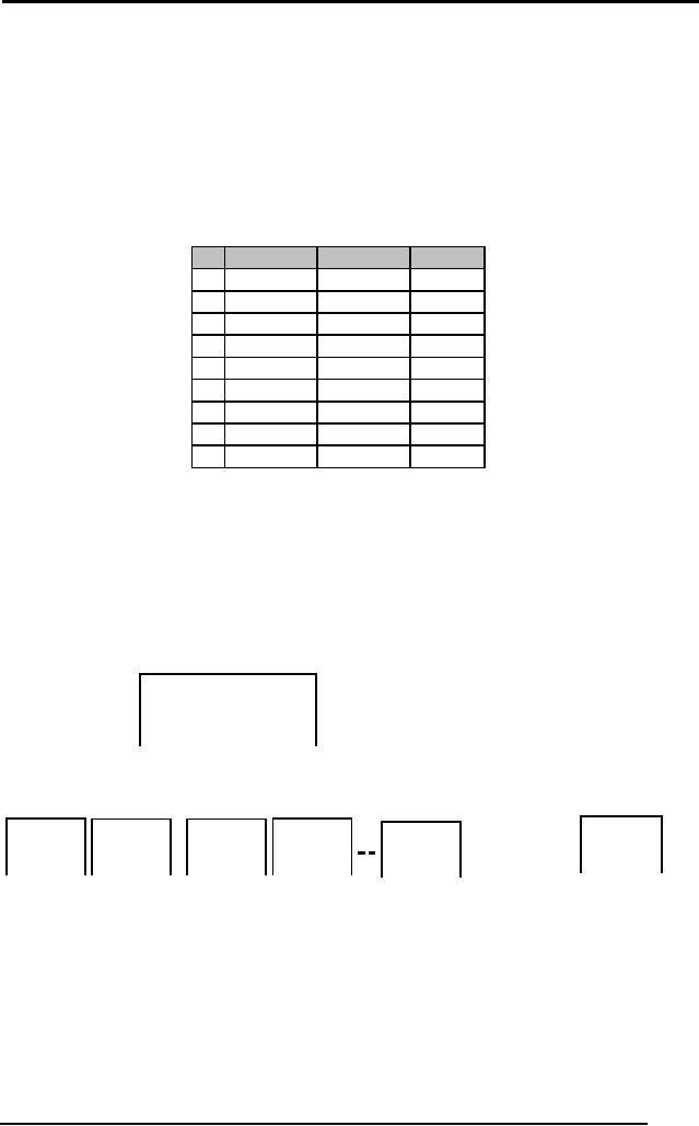
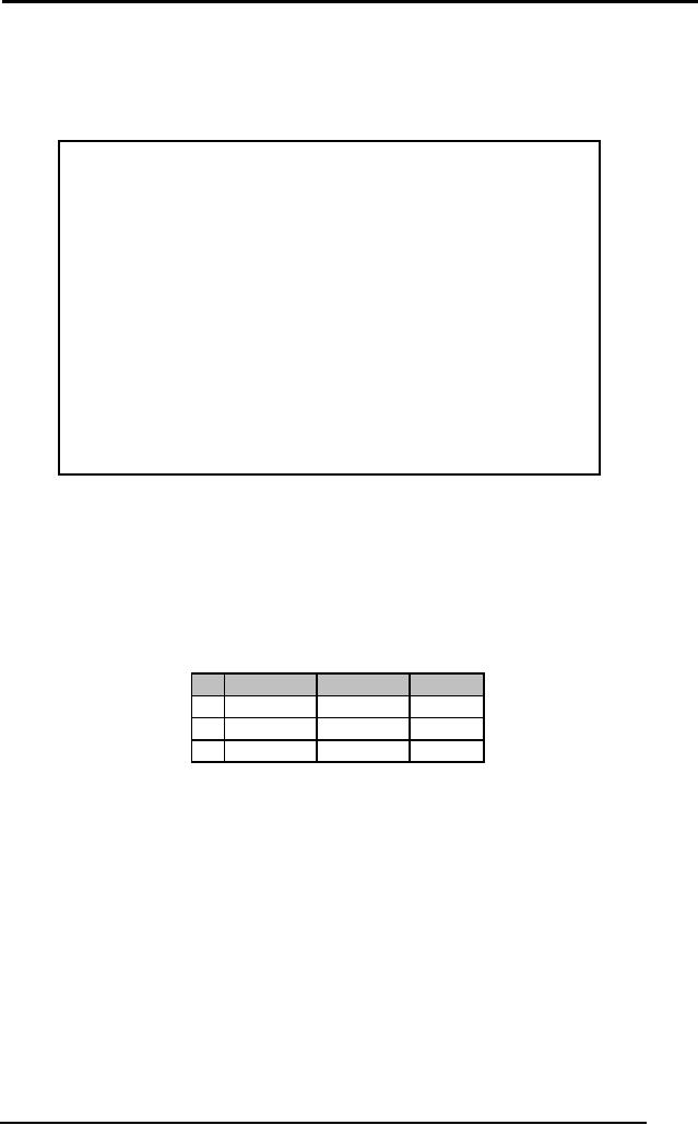
The representation
used here is that every
box in the following diagram
is
populated
using C(xi),
i.e. the value that
the concept C gives as
output when xi is
given to it as
input.
C(x3) C(x6)
C(x9)
C(x2) C(x5)
C(x8)
C(x1) C(x4)
C(x7)
Since we
don't know the concept
yet, so there might be
concepts which can
produce
29 different
outputs, such as:
111
000
000
000
000
111
111
000
100
000
100
111
000
100
100
000
111
111
C29
C1
C2
C3
C4
C29
Each of
these is a different concept,
only one of which is the
true concept (that
we are
trying to learn), but the
dilemma is that we don't
know which one of the 29
is the
true concept of SICK that
we're looking for, since in
real world problems
we
don't
have all the instances in
the instance space X,
available to us for learning.
If
we had all
the possible instances
available, we would know the
exact concept,
but
the problem is that we might
just have three or four
examples of instances
available to us
out of nine.
167

Artificial
Intelligence (CS607)
D
T
BP
SK
x1
N
L
1
x2
L
N
0
x3
N
N
0
Notice
that this is not the
instance space X, in fact it is D:
the training set. We
don't
have any idea about the
instances that lie outside
this set D. The learner
is
to learn
the true concept C based on
only these three
observations, so that
once
it has
learnt, it could classify
the new patients as sick or
healthy based on the
input
parameters.
7.10.3
Hypothesis
space
The above
condition is typically the
case in almost all the
real world problems
where
learning is to be done based on a
few available examples. In
this situation,
the
learner has to hypothesize. It
would be insensible to exhaustively
search over
the
entire concept space, since
there are 29 concepts. This is just a
toy problem
with
only 9 possible instances in
the instance space; just
imagine how huge
the
concept
space would be for real
world problems that involve
larger attribute
sets.
So the
learner has to apply some
hypothesis, which has either
a search or the
language
bias to reduce the size of
the concept space. This
reduced concept
space
becomes the hypothesis
space. For example, the
most common language
bias is
that the hypothesis space
uses the conjunctions (AND)
of the attributes,
i.e.
H = <T,
BP>
H is the
denotive representation of the
hypothesis space; here it is
the
conjunction of
attribute T and BP. If
written in English it would
mean:
H = <T,
BP>:
IF "Temperature" =
T AND "Blood Pressure" = BP
THEN
H=1
ELSE
H=0
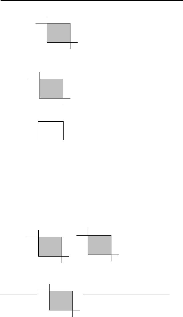
Now if we fill in
these two blanks with
some particular values of T and B, it
would
form a
hypothesis, e.g. for T = N
and BP = N:
168
Artificial
Intelligence (CS607)
BP
H000
N010
L 000
LNH T
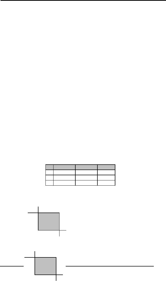
For h =
<L, L>:
BP
H000
N000
L 100
LNH T
Notice
that this is the C2 we presented before in the
concept space
section:
0
0
0
0
0
0
1
0
0
This
means that if the true
concept of SICK that we
wanted to learn was c2 then
the
hypothesis h = <L, L> would
have been the solution to
our problem. But you
must
still be wondering what's
all the use of having
separate conventions
for
hypothesis and
concepts, when in the end we
reached at the same thing:
C2 =
<L, L> = h.
Well, the advantage is that
now we are not required to
look at 29
different
concepts, instead we are
only going to have to look
at the maximum of
17 different
hypotheses before reaching at
the concept. We'll see in a
moment
how
that is possible.
We said H =
<T, BP>. Now T and BP here
can take three values
for sure: L, N
and H, but
now they can take
two more values: ? and Ø.
Where ? means that
for
any value, H = 1,
and Ø means that there
will be no value for which H
will be 1.
For
example, h1
= <?,
?>: [For any value of T
or BP, the person is
sick]
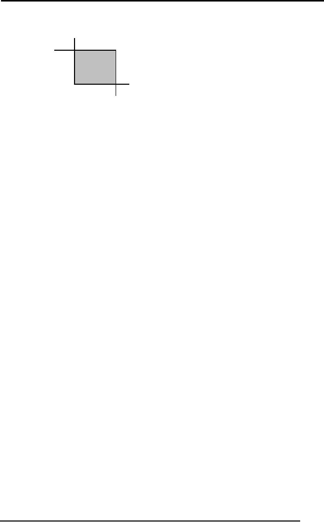
Similarly
h2 = <?, N>:
[For any value of T AND for BP = N,
the person is sick]
BP
BP
H
00
0
H111
N
11
1
N111
L
00
0
L 111
LN
H T
LNH T
h3 = < Ø , Ø >: [For no value of T or
BP, the person
[ is
sick]
BP
169
H
000
N
000
L
000
LNH T
Artificial
Intelligence (CS607)
Having
said all this, how
does this still reduce
the hypothesis space to 17?
Well
it's
simple, now each attribute T
and BP can take 5 values
each: L, N, H, ? and
Ø. So there
are 5 x 5 = 25 total hypotheses
possible. This is a
tremendous
reduction
from 29
= 512 to
25.
But if we
want to represent h4 = < Ø ,
L>, it would be the same
as h3, meaning
that
there are some redundancies
within the 25 hypotheses.
These redundancies
are
caused by Ø, so if there's this
`Ø' in the T or the BP or
both, we'll have
the
same
hypothesis h3
as the
outcome, all zeros. To
calculate the number
of
semantically
distinct hypotheses, we need
one hypothesis which outputs
all
zeros,
since it's a distinct
hypothesis than others, so
that's one, plus we need
to
know
the rest of the
combinations. This primarily
means that T and BP can
now
take 4
values instead of 5, which
are: L, N, H and ?. This implies
that there are
now 4 x 4 = 16
different hypotheses possible. So
the total distinct
hypotheses
are: 16 + 1 =
17. This is a wonderful
idea, but it comes at a
vital cost. What if
the
true
concept doesn't lie in the
conjunctive hypothesis space?
This is often the
case. We
can try different hypotheses
then. Some prior knowledge
about the
problem
always helps.
7.10.4
Version space and
searching
Version
space is a set of all the
hypotheses that are
consistent with all
the
training
examples. When we are given
a set of training examples D, it is
possible
that
there might be more than one
hypotheses from the
hypothesis space that
are
consistent
with all the training
examples. By consistent
we
mean h(xi) =
C(xi).
That
is, if the true output of a
concept [c(xi)] is
1 or 0 for an instance, then
the
output by
our hypothesis [h(xi)] is
1 or 0 as well, respectively. If this is
true for
every
instance in our training set
D, we can say that the
hypothesis is consistent.
Let us
take the following training
set D:
D
T
BP
SK
x1
H
H
1
x2
L
L
0
x3
N
N
0
One of
the consistent hypotheses
can be h1=<H, H >
But
then there are other
hypotheses consistent with D,
such as h2
= < H, ?
>
BP
H00 1
N0 0 0
L 0 00
LNH T
Although it
classifies some of the
unseen instances that are
not in the training
set
BP
H00 1
170
N0 0 1
L 0 01
LNH T
Artificial
Intelligence (CS607)
D, different
from h1, but it's
still consistent over all
the instances in D.
Similarly
BP
H11 1
N0 0 0
L 0 00
LNH T
there's
another hypothesis, h3 = < ?, H >
Notice
the change in h3 as
compared to h2,
but this is again consistent
with D.
Version
space is denoted as VS H,D = {h1, h2, h3}. This
translates as:
Version
space is a
subset of hypothesis space H,
composed of h1, h2 and h3,
that
is
consistent
with D.
7.11
Concept learning as
search
Now that we
are well familiar with
most of the terminologies of
machine learning,
we can
define the learning process
in technical terms
as:
"We have to
assume that the concept
lies in the hypothesis
space. So we search
for a
hypothesis belonging to this
hypothesis space that best
fits the training
examples,
such that the output
given by the hypothesis is
same as the true
output of
concept."
In
short:-
Assume
C∈
H, search
for
an h∈
H
that best fits D
Such
that ∀ xi∈ D, h(xi) =
C(xi).
The stress
here is on the word
`search'. We need to somehow
search through the
hypothesis
space.
7.11.1
General to
specific ordering of hypothesis space
Many algorithms
for concept learning
organize the search through
the hypothesis
space by
relying on a very useful
structure that exists for
any concept learning
problem: a
general-to-specific ordering of
hypotheses. By taking advantage
of
this
naturally occurring structure
over the hypothesis space,
we can design
learning
algorithms that exhaustively
search even infinite
hypothesis spaces
without
explicitly enumerating every
hypothesis. To illustrate the
general-to-
specific
ordering, consider two
hypotheses:
h1 = < H, H
>
h2 = < ?, H
>
Now consider
the sets of instances that
are classified positive by h1
and by h2.
Because h2
imposes fewer constraints on
the instance, it classifies
more
instances as
positive. In fact, any
instance classified positive by h1
will also be
classified
positive by h2. Therefore, we
say that h2 is more general
than h1.
So all
the hypothesis in H can be
ordered according to their
generality, starting
from < ?, ?
> which is the most
general hypothesis since it
always classifies all
171

Artificial
Intelligence (CS607)
the
instances as positive. On the
contrary we have < Ø , Ø > which is
the most
specific
hypothesis, since it doesn't
classify a single instance as
positive.
7.11.2
FIND-S
FIND-S
finds the maximally specific
hypothesis possible within
the version space
given a
set of training data. How
can we use the general to
specific ordering of
hypothesis
space to organize the search
for a hypothesis consistent
with the
observed
training examples? One way is to begin
with the most specific
possible
hypothesis in H,
then generalize the
hypothesis each time it
fails to cover an
observed
positive training example.
(We say that a hypothesis
"covers" a positive
example if it
correctly classifies the
example as positive.) To be more
precise
about
how the partial ordering is
used, consider the FIND-S
algorithm:
Initialize
h to the
most specific hypothesis in H
For
each positive training
instance x
For
each attribute constraint ai in
h
If the
constraint ai is
satisfied by x
Then do
nothing
Else
Replace
ai in
h by the
next more general
constraint
that is satisfied by x
Output
hypothesis h
To illustrate
this algorithm, let us
assume that the learner is
given the sequence
of following
training examples from the
SICK domain:
D
T
BP
SK
x1
H
H
1
x2
L
L
0
x3
N
H
1
The first
step of FIND-S is to initialize
h to the
most specific hypothesis in H:
h=<Ø,Ø>
Upon observing
the first training example
(< H, H >, 1), which happens to be
a
positive
example, it becomes obvious
that our hypothesis is too
specific. In
particular,
none of the "Ø" constraints
in h are
satisfied by this training
example,
so each Ø is
replaced by the next more
general constraint that fits
this particular
example;
namely, the attribute values
for this very training
example:
h=<H,H>
This is
our h
after
we have seen the first
example, but this h is still
very specific. It
asserts
that all instances are
negative except for the
single positive
training
example we
have observed.
Upon encountering
the second example; in this
case a negative example,
the
algorithm
makes no change to h. In fact,
the FIND-S
algorithm simply
ignores
every
negative example. While
this may at first seem
strange, notice that in
the
current
case our hypothesis h is already
consistent with the new
negative
example
(i.e. h correctly
classifies this example as
negative), and hence no
revision is
needed. In the general case,
as long as we assume that
the
hypothesis
space H contains a
hypothesis that describes
the true target
concept
172

Artificial
Intelligence (CS607)
c and
that the training data
contains no errors and
conflicts, then the
current
hypothesis
h can
never require a revision in
response to a negative
example.
To complete
our trace of FIND-S, the
third (positive) example
leads to a further
generalization of
h, this
time substituting a "?" in
place of any attribute value
in h
that is
not satisfied by the new
example. The final hypothesis
is:
h = < ?, H
>
This
hypothesis will term all
the future patients which
have BP = H as SICK for
all
the
different values of T.
There
might be other hypotheses in
the version space but
this one was
the
maximally
specific with respect to the
given three training
examples. For
generalization
purposes we might be interested in
the other hypotheses
but
FIND-S
fails to find the other
hypotheses. Also in real
world problems, the
training
data
isn't consistent and void of
conflicting errors. This is
another drawback of
FIND-S,
that, it assumes the
consistency within the
training set.
7.11.3
Candidate-Elimination
algorithm
Although
FIND-S outputs a hypothesis
from H that is consistent
with the training
examples,
but this is just one of many
hypotheses from H that might
fit the
training
data equally well. The key idea in
Candidate-Elimination algorithm is
to
output a
description of the set of
all hypotheses consistent
with the training
examples. This
subset of all hypotheses is
actually the version
space with
respect to
the hypothesis space H and the
training examples D, because
it
contains
all possible versions of the
target concept.
The
Candidate-Elimination algorithm
represents the version space
by storing only
its
most general members
(denoted by G) and its
most specific members
(denoted by
S). Given
only these two sets
S and G, it is possible
to enumerate all
members of
the version space as needed
by generating the hypotheses
that lie
between
these two sets in
general-to-specific partial ordering
over hypotheses.
Candidate-Elimination
algorithm begins by initializing
the version space to the
set
of all
hypotheses in H; that is by
initializing the G boundary
set to contain the
most
general hypothesis in H, for
example for the SICK
problem, the G0 will
be:
G0 = {< ?, ? >}
The S boundary
set is also initialized to
contain the most specific
(least general)
hypothesis:
S0 = {< Ø , Ø >}
These
two boundary sets (G and S) delimit
the entire hypothesis space,
because
every
other hypothesis in H is both
more general than S0 and
more specific than
G0. As
each training example is
observed one by one, the
S boundary is
made
more
and more general, whereas
the G
boundary
set is made more and
more
specific, to
eliminate from the version
space any hypotheses found
inconsistent
with
the new training example.
After all the examples
have been processed,
the
computed
version space contains all
the hypotheses consistent
with these
examples. The
algorithm is summarized
below:
173
Artificial
Intelligence (CS607)
Initialize
G to the
set of maximally general
hypotheses in H
Initialize
S to the
set of maximally specific
hypotheses in H
For
each training example d, do
If d is a positive
example
Remove
from G any
hypothesis inconsistent with d
For
each hypothesis s in S that is
inconsistent with d
Remove
s from S
Add to
S all
minimal generalization h of s, such
that
h is consistent
with d, and
some member of G is more
general than h
Remove
from S any
hypothesis that is more
general than another one in
S
If d is a negative
example
Remove
from S any
hypothesis inconsistent with d
For
each hypothesis g in G that is
inconsistent with d
Remove
g from G
Add to
G all
minimal specializations h of g, such
that
h is consistent
with d, and
some member of S is more
specific than h
Remove
from G any
hypothesis that is less
general than another one in
S
The
Candidate-Elimination algorithm above is
specified in terms of
operations.
The detailed
implementation of these operations
will depend on the
specific
problem and
instances and their
hypothesis space, however
the algorithm can be
applied to any
concept learning task. We
will now apply this
algorithm to our
designed
problem SICK, to trace the
working of each step of the
algorithm. For
comparison
purposes, we will choose the
exact training set that
was employed in
FIND-S:
D
T
BP
SK
x1
H
H
1
x2
L
L
0
x3
N
H
1
We know
the initial values of G and
S:
G0 = {< ?, ? >}
S0 = {< Ø, Ø >}
Now the
Candidate-Elimination learner
starts:
First
training observation is: d1 = (<H, H>, 1) [A positive
example]
G1 = G0 = {< ?, ? >},
since <?, ?> is consistent
with d1;
both give positive
outputs.
Since
S0 has only
one hypothesis that is < Ø, Ø >,
which implies S0(x1) = 0, which
is not
consistent with d1, so we
have to remove < Ø, Ø > from
S1. Also, we
add
minimally
general hypotheses from H to
S1, such that
those hypotheses are
consistent
with d1.
The obvious choices are
like <H,H>, <H,N>,
<H,L>,
174

Artificial
Intelligence (CS607)
<N,H>.........
<L,N>, <L,L>, but
none of these except
<H,H> is consistent with
d1.
So S1 becomes:
S1 = {< H, H >}
G1 = {< ?, ? >}
Second
training example is: d2 = (<L, L>, 0) [A negative
example]
S2 = S1 = {< H, H>},
since <H, H> is consistent
with d2: both give
negative outputs
for x2.
G1 has only one hypothesis:
< ?, ? >, which gives a positive
output on x2,
and
hence is
not consistent, since
SK(x2) = 0, so we have to
remove it and add in its
place,
the hypotheses which are
minimally specialized. While
adding we have to
take
care of two things; we would
like to revise the statement
of the algorithm for
the
negative examples:
"Add to G all
minimal specializations h of g, such
that
h is consistent
with d, and some member of
S is more specific
than h"
The immediate one
step specialized hypotheses of < ?, ?
> are:
{< H, ? >, < N, ?
>, < L, ? >, < ?, H >, < ?, N >, < ?, L
>}
Out of
these we have to get rid of
the hypotheses which are
not consistent with d2
= (<L,
L>, 0). We see that
all of the above listed
hypotheses will give a
0
(negative)
output on x2
= < L, L >,
except for < L, ? > and < ?, L
>, which give a 1
(positive)
output on x2,
and hence are not
consistent with d2, and
will not be
added to
G2. This leaves us
with {< H, ? >, < N, ? >, < ?, H >, < ?, N
>}. This
takes
care of the inconsistent
hypotheses, but there's
another condition in
the
algorithm
that we must take care of
before adding all these
hypotheses to G2.
We
will
repeat the statement again,
this time highlighting the
point under
consideration:
"Add to G all
minimal specializations h of g, such
that
h is consistent
with d, and some member of S is more specific
than h"
This is
very important condition,
which is often ignored, and
which results in the
wrong
final version space. We know
the current S we have is S2, which is: S2 = {<
H, H>}. Now
for which hypotheses do you
think < H, H > is more specific
to, out
of {< H, ? >, < N, ?
>, < ?, H >, < ?, N >}. Certainly <
H, H > is more specific
than
< H, ? > and
< ?, H >, so we remove < N, ? > and < ?, N
>to get the final
G2:
G2 = {< H, ? >, < ?, H >}
S2 = {< H, H>}
Third and
final training example is:
d3 = (<N, H>, 1) [A positive
example]
We see
that in G2, < H, ?
> is not consistent with d3, so we remove it:
G3 = {< ?, H >}
175
Artificial
Intelligence (CS607)
We also
see that in S2, < H, H > is
not consistent with d3, so we remove it and
add minimally
general hypotheses than < H, H >.
The two choices we have
are: <
H, ? > and < ?, H >.
We only keep < ?, H >, since
the other one is not
consistent
with d3. So our final version
space is encompassed by S3 and G3:
G3 = {< ?, H >}
S3 = {< ?, H >}
It is only a
coincidence that both G and
S sets are the same. In
bigger problems,
or even
here if we had more examples,
there was a chance that
we'd get different
but
consistent sets. These two
sets of G and S outline the
version space of a
concept.
Note that the final
hypothesis is the same one
that was computed by
FIND-S.
7.12
Decision trees
learning
Up until
now we have been searching
in conjunctive spaces which
are formed by
ANDing
the attributes, for
instance:
IF Temperature =
High AND Blood
Pressure = High
THEN Person =
SICK
But
this is a very restrictive
search, as we saw the
reduction in hypothesis
space
from 29 total possible concepts to
17. This can be risky if
we're not sure if the
true
concept
will lie in the conjunctive
space. So a safer approach is to
relax the
searching
constraints. One way is to
involve OR into the search.
Do you think
we'll
have a bigger search space
if we employ OR? Yes, most
certainly; consider,
for
example, the
statement:
IF Temperature =
High OR Blood
Pressure = High
THEN Person =
SICK
If we could
use these kind of OR
statements, we'd have a
better chance of
finding
the true concept, if the
concept does not lie in
the conjunctive
space.
These
are also called disjunctive
spaces.
7.12.1
Decision tree
representation
Decision
trees give us disjunctions of
conjunctions, that is, they
have the form:
(A AND B) OR (C AND
D)
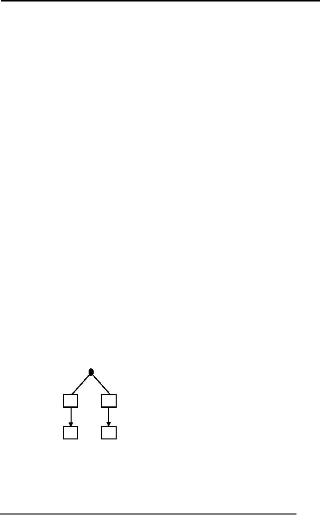
In tree
representation, this would
translate into:
A
C
B
D
where A, B, C
and D are the attributes
for the problem. This
tree gives a positive
output if
either A AND B attributes are
present in the instance; OR C AND
D
attributes
are present. Through
decision trees, this is how
we reach the final
hypothesis.
This is a hypothetical tree. In
real problems, every tree
has to have a
176

Artificial
Intelligence (CS607)
root
node. There are various
algorithms like ID3 and C4.5 to
find decision trees
for
learning problems.
7.12.2
ID3
ID stands
for interactive dichotomizer.
This was the 3rd revision of the
algorithm
which
got wide acclaims. The
first step of ID3 is to find
the root node. It uses
a
special
function GAIN, to evaluate the
gain information of each
attribute. For
example if
there are 3 instances, it
will calculate the gain
information for each.
Whichever
attribute has the maximum
gain information, becomes
the root node.
The rest of
the attributes then fight
for the next
slots.
7.12.2.1
Entropy
In order to
define information gain
precisely, we begin by defining a
measure
commonly
used in statistics and information
theory, called entropy,
which
characterizes
the purity/impurity of an arbitrary
collection of examples. Given
a
collection S,
containing positive and negative
examples of some target
concept,
the
entropy of S relative to this
Boolean classification
is:
Entropy(S) = -
p+log2 p+ - p-log2 p-
where
p+ is the proportion
of positive examples in S and p- is the proportion of
negative
examples in S. In all calculations
involving entropy we define
0log 0 to
be 0.
To illustrate,
suppose S is a collection of 14 examples
of some Boolean
concept,
including 9
positive and 5 negative
examples, then the entropy
of S relative to
this
Boolean classification
is:
Entropy(S) = -
(9/14)log2
(9/14) -
(5/14)log2
(5/14)
=
0.940
Notice
that the entropy is 0, if
all the members of S belong
to the same class
(purity).
For example, if all the
members are positive (p+ = 1),
then p- = 0 and
so:
Entropy(S) = -
1log2 1 - 0log2 0
= - 1 (0) -
0
[since
log2 1 = 0, also
0log2 0 = 0]
=0
Note
the entropy is 1 when the
collection contains equal
number of positive and
negative
examples (impurity). See for
yourself by putting p+ and p- equal to
1/2.
Otherwise if
the collection contains
unequal numbers of positive and
negative
examples,
the entropy is between 0 and
1.
7.12.2.2
Information
gain
Given
entropy as a measure of the
impurity in a collection of training
examples,
we can
now define a measure of the
effectiveness of an attribute in
classifying
the
training data. The measure we
will use, called information
gain,
is simply the
expected
reduction in entropy caused by
partitioning the examples
according to
this
attribute. That is, if we
use the attribute with
the maximum information
gain
as the
node, then it will classify
some of the instances as
positive or negative
with
100%
accuracy, and this will
reduce the entropy for
the remaining instances.
We
will
now proceed to an example to
explain further.
177

Artificial
Intelligence (CS607)
7.12.2.3
Example
Suppose we
have the following
hypothetical training data
available to us given in
the
table below. There are
three attributes: A, B and E.
Attribute A can take
three
values:
a1, a2 and
a3. Attribute B can
take two values: b1 and b2. Attribute E
can
also
take two values: e1 and e2. The
concept to be learnt is a Boolean
concept,
so C takes a YES
(1) or a NO (0), depending on
the values of the
attributes.
S
A
B
E
C
d1
a1
b1
e2
YES
d2
a2
b2
e1
YES
d3
a3
b2
e1
NO
d4
a2
b2
e1
NO
d5
a3
b1
e2
NO
First
step is to calculate the
entropy of the entire set S.
We know:
E(S) = - p+log2 p+ - p-log2 p-
2
2 2
3
- log
2 - log
2 =
0.97
5
5 5
5
We have
the entropy of the entire
training set S with us now.
We have to
calculate
the information gain for
each attribute A, B, and E based on
this entropy
so that
the attribute giving the
maximum information is to be placed at
the root of
the
tree.
The formula
for calculating the gain
for A is:
| Sa1 |
| Sa2 |
| Sa3 |
G(S , A) = E(S ) -
E (Sa1 ) -
E (Sa2 ) -
E(Sa3 )
|S|
|S|
|S|
where |Sa1| is
the number of times
attribute A takes the value
a1.
E(Sa1) is
the
entropy of
a1,
which will be calculated by
observing the proportion of
total
population of
a1 and
the number of times the C is
YES or NO within these
observation
containing a1 for
the value of A.
For
example, from the table it
is obvious that:
|S| = 5
|Sa1| =
1
[since
there is only one observation of
a1 which
outputs a YES]
E(Sa1) =
-1log21 - 0log20 = 0
[since
log 1 = 0]
|Sa2| =
2
[one
outputs a YES and the other
outputs NO]
1
1 1
1
1
1
E(Sa2) =
-
log
2 - log
2 = - (- 1) - (- 1) = 1
2
2 2
2
2
2
|Sa3| =
1
[since
there is only one observation of
a3 which
outputs a NO]
E(Sa3) =
-0log20 - 1log21 = 0
[since
log 1 = 0]
Putting
all these values in the
equation for G(S,A)
we
get:
178
Artificial
Intelligence (CS607)
1
(0) - 2 (1) - 1 (0) =
0.57
G(S , A) = 0.97 -
5
5
5
Similarly
for B, now since there
are only two values
observable for the attribute
B:
| Sb2 |
| Sb1 |
G(S , B) = E(S ) -
E(Sb1 ) -
E(Sb2 )
|S|
|S|
2
3 1
1 2
2
G(S , B) = 0.97 - (1) - (- log
2 - log
2 )
5
5 3
3 3
3
3
G(S , B) = 0.97 - 0.4 - (0.52 + 0.39) =
0.02
5
Similarly
for E
| Se1 |
| Se2 |
E(Se2 ) =
0.02
G(S , E ) = E(S ) -
E (Se1 ) -
|S|
|S|
This
tells us that information
gain for A is the highest.
So we will simply choose
A
as the
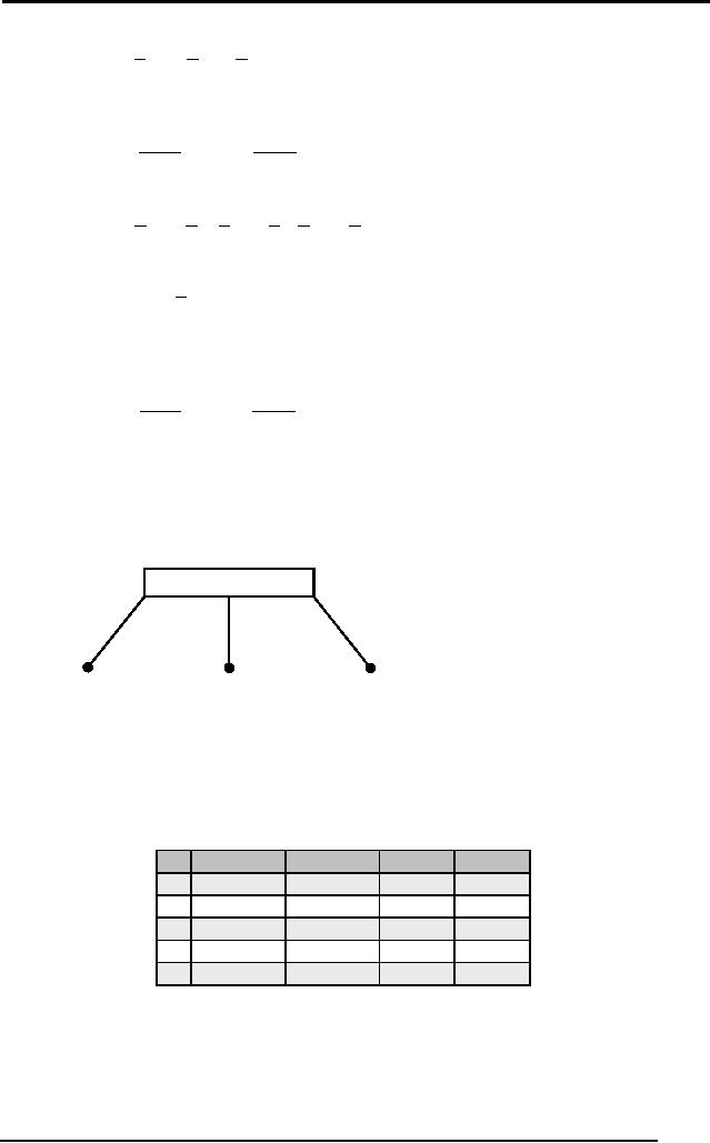
root of our decision tree.
By doing that we'll check if
there are any
conflicting
leaf nodes in the tree.
We'll get a better picture
in the pictorial
representation
shown below:
A
a1
a2
a3
YES
S' = [d2, d4]
NO
This is a
tree of height one, and we
have built this tree
after only one
iteration.
This
tree correctly classifies 3
out of 5 training samples,
based on only one
attribute A,
which gave the maximum
information gain. It will
classify every
forthcoming
sample that has a value of
a1 in attribute A as
YES, and each sample
having
a3 as NO. The
correctly classified samples
are highlighted
below:
S
A
B
E
C
d1
a1
b1
e2
YES
d2
a2
b2
e1
YES
d3
a3
b2
e1
NO
d4
a2
b2
e1
NO
d5
a3
b1
e2
NO
Note
that a2
was
not a good determinant for
classifying the output C,
because it
gives
both YES and NO for d2 and d4
respectively.
This means that now we
have
to look at
other attributes B and E to
resolve this conflict. To
build the tree
further
we will
ignore the samples already
covered by the tree above.
Our new sample
space
will be given by S' as given in
the table below:
179

Artificial
Intelligence (CS607)
S' A
B
E
C
d2 a2
B2
e1
YES
d4 a2
B2
e2
NO
We'll
apply the same process as
above again. First we
calculate the entropy
for
this
sub sample space
S':
E(S') = - p+log2 p+ - p-log2 p-
1
1 1
1
= - log
2 - log
2 =
1
2
2 2
2
This
gives us entropy of 1, which is
the maximum value for
entropy. This is also
obvious
from the data, since
half of the samples are
positive (YES) and half
are
negative
(NO).
Since
our tree already has a
node for A, ID3 assumes that
the tree will not
have
the
attribute repeated again,
which is true since A has
already divided the data
as
much as it
can, it doesn't make any
sense to repeat A in the
intermediate nodes.
Give
this a thought yourself too.
Meanwhile, we will calculate
the gain information
of B and E
with respect to this new
sample space S':
|S'| = 2
|S'b2| =
2
| S ' b2 |
G(S ' , B) = E (S ' ) -
E (S ' b2 )
| S '|
2 1
1 1
1
G(S ' , B) = 1 - (- log
2 - log
2 ) = 1 - 1 = 0
2 2
2 2
2
Similarly
for E:
|S'| = 2
|S'e1| =
1
[since
there is only one observation of
e1 which
outputs a YES]
E(S'e1) =
-1log21 - 0log20 = 0
[since
log 1 = 0]
|S'e2| =
1
[since
there is only one observation of
e2 which
outputs a NO]
E(S'e2) =
-0log20 - 1log21 = 0
[since
log 1 = 0]
Hence:
| S ' e1 |
| S ' e2 |
G(S ' , E ) = E (S ' ) -
E (S ' e1 ) -
E (S ' e2 )
| S '|
| S '|
1
1
G(S ' , E ) = 1 - (0) - (0) = 1 - 0 - 0 =
1
2
2
Therefore E
gives us a maximum information
gain, which is also true
intuitively
since by
looking at the table for
S', we can see that B
has only one value b2,
which
doesn't help us decide
anything, since it gives
both, a YES and a NO.
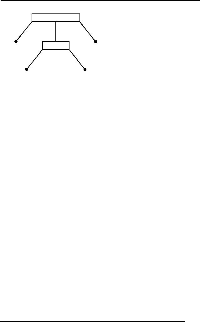
Whereas, E
has two values, e1 and e2; e1 gives a YES and e2 gives a NO. So we
put
the node E in the tree
which we are already
building. The
pictorial
representation is
shown below:
180
Artificial
Intelligence (CS607)
A
a1
a2
a3
YES
NO
E
e1
e2
YES
NO
Now we will
stop further iterations
since there are no
conflicting leaves that
we
need to
expand. This is our
hypothesis h that
satisfies each training
example.
7.13
LEARNING: Connectionist
Although ID3
spanned more of the concept
space, but still there is a
possibility
that
the true concept is not
simply a mixture of disjunctions of
conjunctions, but
some
more
complex
arrangement
of
attributes.
(Artificial
Neural Networks) ANNs can
compute more complicated
functions
ranging
from linear to any higher
order quadratic, especially
for non-Boolean
concepts.
This new learning paradigm
takes its roots from
biology inspired
approach to
learning. Its primarily a
network of parallel distributed
computing in
which
the focus of algorithms is on
training rather than
explicit programming.
Tasks
for which connectionist
approach is well suited
include:
· Classification
· Fruits
Apple or orange
· Pattern
Recognition
· Finger
print, Face
recognition
· Prediction
· Stock
market analysis, weather
forecast
7.14
Biological aspects and structure of a
neuron
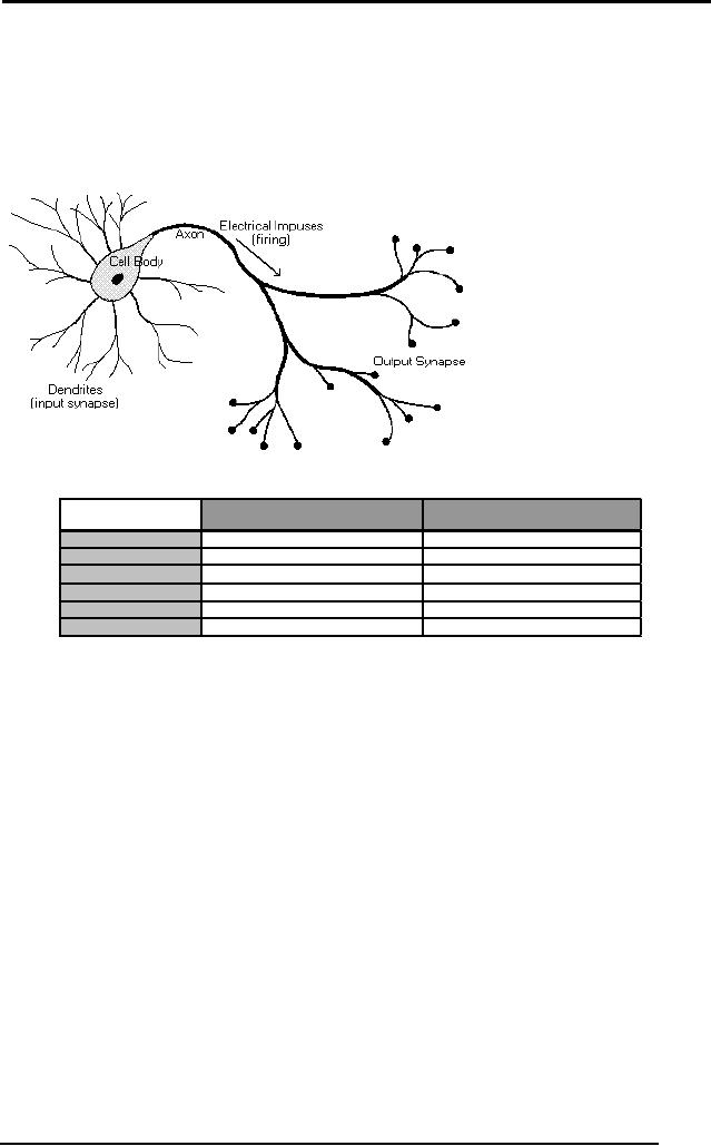
The brain is a
collection of about 100 billion
interconnected neurons.
Each
neuron is a
cell that uses biochemical
reactions to receive, process and
transmit
information. A
neuron's dendritic tree is
connected to a thousand
neighboring
neurons.
When one of those neurons
fire, a positive or negative
charge is
received by one of
the dendrites. The strengths
of all the received charges
are
added
together through the
processes of spatial and
temporal summation.
Spatial
summation
occurs when several weak
signals are converted into a
single large
one,
while temporal summation
converts a rapid series of
weak pulses from
one
source
into one large signal. The
aggregate input is then
passed to the soma
(cell
body). The
soma and the enclosed
nucleus don't play a
significant role in
the
processing of
incoming and outgoing data.
Their primary function is to
perform
the
continuous maintenance required to
keep the neuron functional.
The part of
the
soma that does concern
itself with the signal is
the axon hillock. If
the
aggregate
input is greater than the
axon hillock's threshold
value, then the
neuron
fires, and an
output signal is transmitted
down the axon. The
strength of the
output is
constant, regardless of whether
the input was just
above the threshold,
or a hundred
times as great. The output
strength is unaffected by the
many
181
Artificial
Intelligence (CS607)
divisions in
the axon; it reaches each
terminal button with the
same intensity it
had at the
axon hillock. This
uniformity is critical in an analogue
device such as a
brain
where small errors can
snowball, and where error
correction is more
difficult
than in a
digital system. Each
terminal button is connected to
other neurons
across a
small gap called a
synapse.
7.14.1
Comparison between computers
and the brain
Biological
Neural Networks
Computers
Speed
Fast
(nanoseconds)
Slow
(milliseconds)
Processing
Superior
(massively parallel)
Inferior
(Sequential mode)
1011 neurons, 1015 interconnections
Size &
Complexity
Far
few processing
elements
Storage
Adaptable,
interconnection strengths
Strictly
replaceable
Fault
tolerance
Extremely
Fault tolerant
Inherently
non fault tolerant
Control
mechanism
Distributive
control
Central
control
While
this clearly shows that
the human information
processing system is
superior to
conventional computers, but
still it is possible to realize an
artificial
neural
network which exhibits the
above mentioned properties.
We'll start with a
single
perceptron, pioneering work
done in 1943 by McCulloch and
Pitts.
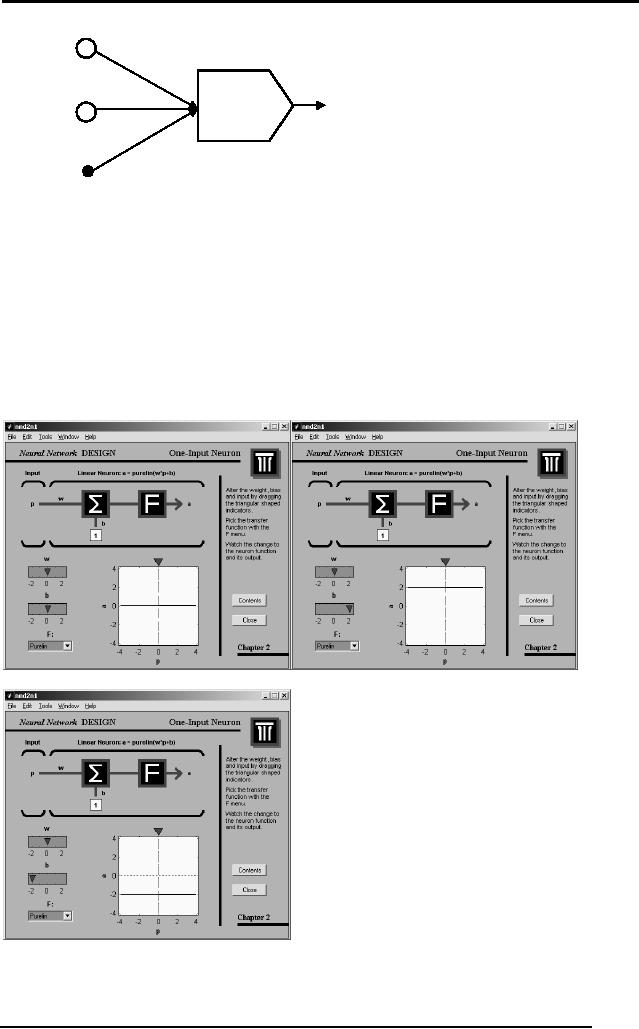
7.15
Single perceptron
To capture
the essence of biological
neural systems, an artificial
neuron is
defined as
follows:
It receives a
number of inputs (either
from original data, or from
the output of
other
neurons in the neural
network). Each input comes
via a connection that
has
a strength
(or weight); these weights
correspond to synaptic efficacy in
a
biological
neuron. Each neuron also
has a single threshold
value. The weighted
sum of
the inputs is formed, and
the threshold subtracted, to
compose the
activation of
the neuron. The activation
signal is passed through an
activation
function
(also known as a transfer
function) to produce the
output of the neuron.
182
Artificial
Intelligence (CS607)
Input1
weigh
Threshold
Output
Input2
Function
weigh
Bias
Neuron
Firing Rule:
IF (Input1 x
weight1) + (Input2 x weight2) +
(Bias) satisfies Threshold
value
Then
Output = 1
Else
Output = 0
7.15.1
Response of changing
bias
The response of
changing the bias of a
neuron results in shifting
the decision line
up or down, as
shown by the following
figures taken from
matlab.
183
Artificial
Intelligence (CS607)
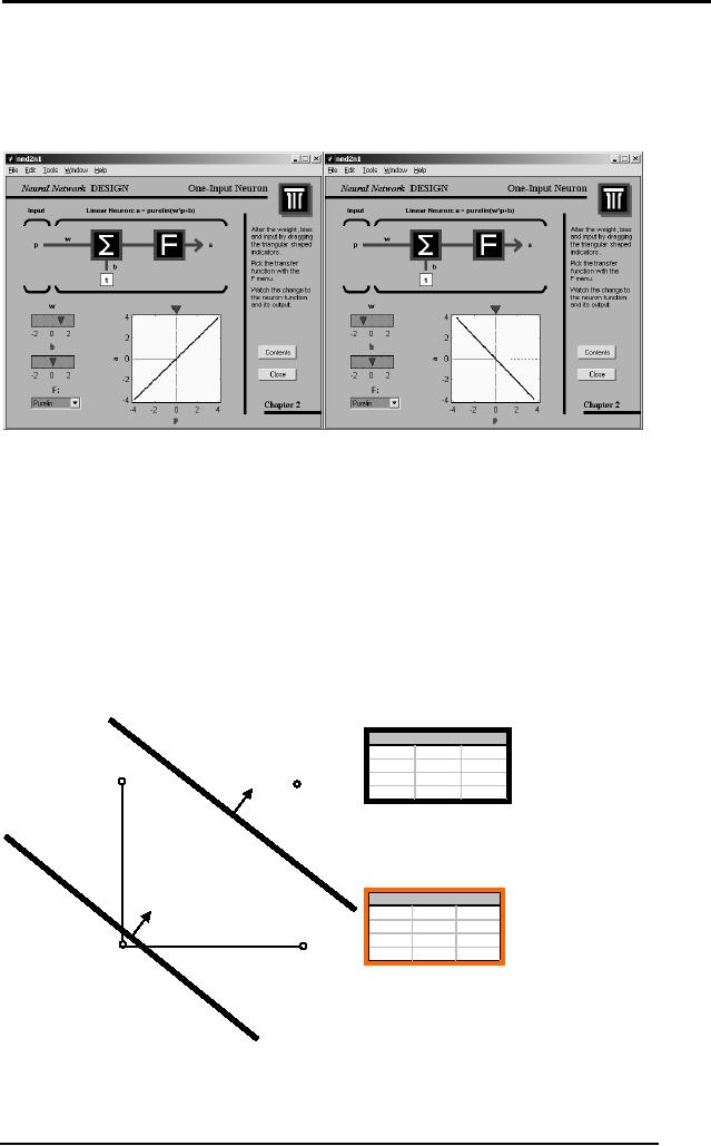
7.15.2
Response of changing
weight
The change in
weight results in the
rotation of the decision
line. Hence this up
and down
shift, together with the
rotation of the straight
line can achieve any
linear
decision.
7.16
Linearly separable problems
There is a
whole class of problems
which are termed as linearly
separable. This
name is
given to them, because if we
were to represent them in
the input space,
we could
classify them using a
straight line. The simplest
examples are the
logical AND or
OR. We have drawn them in
their input spaces, as this
is a simple
2D problem. The
upper sloping line in the
diagram shows the decision
boundary
for AND
gate, above which, the
output is 1, below is 0. The lower
sloping line
decides
for the OR gate
similarly.
Input
1
Input
2
AND
0
0
0
(1,0
(1,1
0
1
0
1
0
0
1
1
1
Input
2
Input
1
Input
2
OR
0
0
0
0
1
1
1
0
1
1
1
1
(0,0)
(0,1
Input
1
A single
perceptron simply draws a
line, which is a hyper plane
when the data is
more
then 2 dimensional. Sometimes
there are complex problems
(as is the case
184
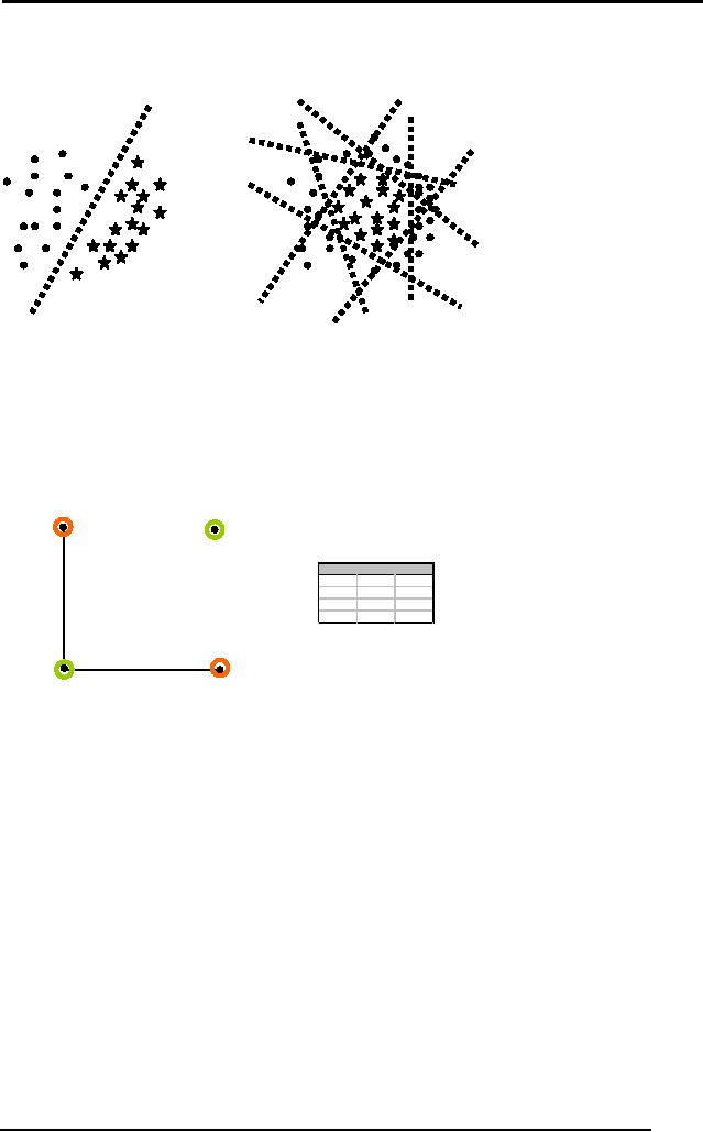
Artificial
Intelligence (CS607)
in real
life). The data for these
problems cannot be separated
into their respective
classes by
using a single straight
line. These problems are
not linearly
separable.
Linearly
Separable
Linearly
Non Separable /
Non
linear decision
region
Another
example of linearly non-separable
problems is the XOR gate
(exclusive
OR).
This shows how such a
small data of just 4 rows,
can make it impossible
to
draw one
line decision boundary,
which can separate the 1s
from 0s.
(1,0)
(1,1)
Input
1
Input
2
Output
0
0
1
Input
2
0
1
0
1
0
0
1
1
1
(0,0)
(0,1)
Input
1
Can
you draw one line
which separates the ones
from zeros for the
output?
185
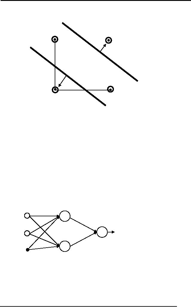
Artificial
Intelligence (CS607)
We need
two lines:
(1,0)
(1,1)
Input
2
(0,0)
(0,1)
Input
1
A single
layer perceptron can perform
pattern classification only on
linearly
separable
patterns, regardless of the
type of non-linearity (hard
limiter, signoidal).
Papert
and Minsky in 1969
illustrated the limitations of
Rosenblatt's single
layer
perceptron
(e.g. requirement of linear
separability, inability to solve
XOR
problem) and
cast doubt on the viability
of neural networks. However,
multi-layer
perceptron and
the back-propagation algorithm
overcomes many of the
shortcomings of
the single layer
perceptron.
7.17
Multiple layers of
perceptrons
Just as in
the previous example we saw
that XOR needs two lines to
separate
the
data without incorporating
errors. Likewise, there are
many problems which
need to
have multiple decision lines
for a good acceptable
solution. Multiple
layer
perceptrons
achieve this task by the
introduction of one or more
hidden layers.
Each
neuron in the hidden layer
is responsible for a different
line. Together they
form a
classification for the given
problem.
Input
1
Input
2
1
Hidden
Output
Input
Layer
Layer
Layer
Each
neuron in the hidden layer
forms a different decision
line. Together all
the
lines
can construct any arbitrary
non-linear decision boundaries.
These multi-
layer
perceptrons are the most
basic artificial neural
networks.
186
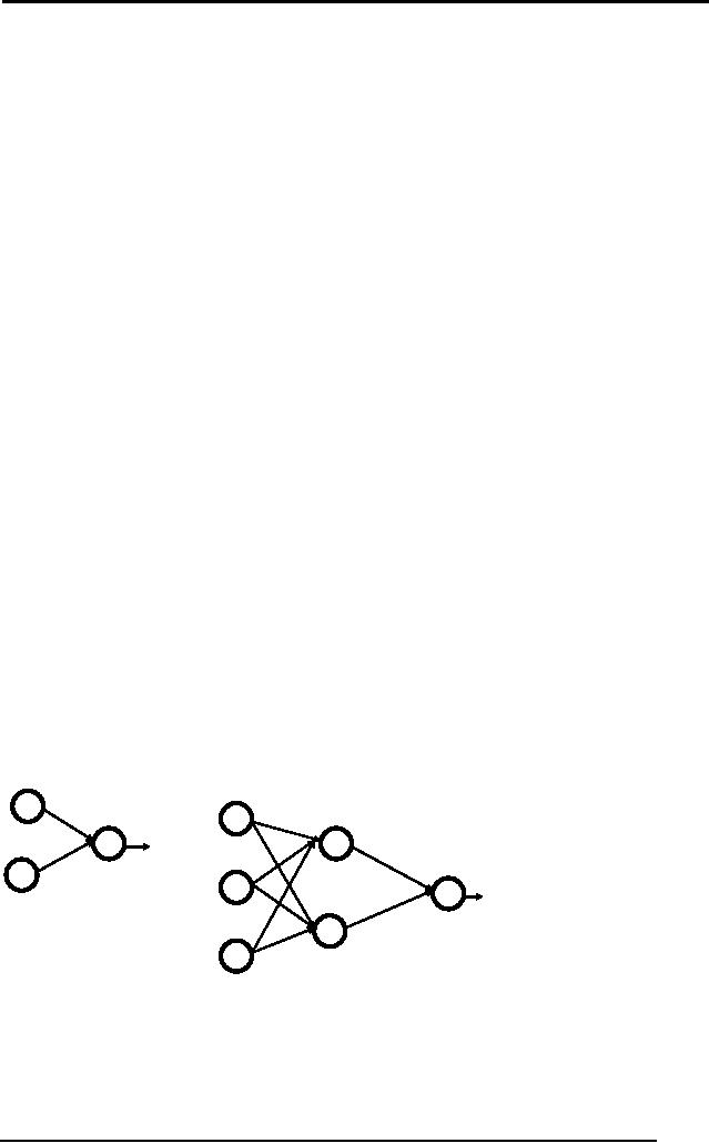
Artificial
Intelligence (CS607)
7.18
Artificial Neural Networks:
supervised and unsupervised
A neural
network is a massively parallel
distributed computing system
that has a
natural
propensity for storing
experiential knowledge and
making it available
for
use. It
resembles the brain in two
respects:
· Knowledge is
acquired by the network
through a learning process
(called
training)
· Interneuron
connection strengths known as
synaptic weights are used
to
store
the knowledge
Knowledge in
the artificial neural
networks is implicit and
distributed.
Advantages
· Excellent
for pattern
recognition
· Excellent
classifiers
· Handles
noisy data well
· Good for
generalization
Draw
backs
· The
power of ANNs lie in their
parallel architecture
Unfortunately,
most machines we have are
serial (Von Neumann
architecture)
· Lack of
defined rules to build a
neural network for a
specific problem
Too many
variables, for instance, the
learning algorithm, number
of
neurons
per layer, number of layers,
data representation
etc
· Knowledge is
implicit
· Data
dependency
But
all these drawbacks doesn't
mean that the neural
networks are useless
artifacts.
They are still arguably
very powerful general
purpose problem
solvers.
7.19 Basic
terminologies
Number of
layers
·
o Single
layer network
o Multilayer
networks
Single
Layer
Two
Layers
Only
one input and
One
input ,
One
hidden and
One
output layer
One
output layer
187
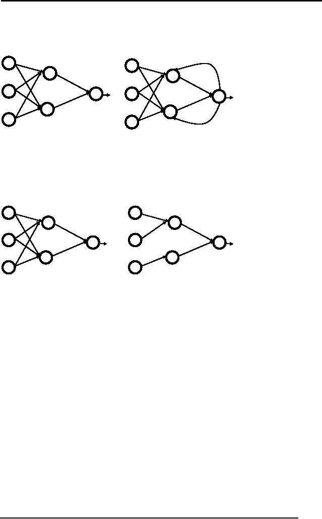
Artificial
Intelligence (CS607)
Direction of
information (signal)
flow
·
o Feed-forward
o Recurrent
(feed-back)
Feed
forward
Recurrent
Network
Connectivity
·
o Fully
connected
o Partially
connected
Fully
connected
Partially
connected
Learning
methodology
·
o Supervised
Given a
set of example input/output
pairs, find a rule that
does a
good
job of predicting the output
associated with a new
input.
o Unsupervised
Given a
set of examples with no
labeling, group them
into
sets
called clusters
Knowledge is
not explicitly represented in
ANNs. Knowledge is primarily
encoded
in the
weights of the neurons
within the network
7.20
Design phases of ANNs
Feature
Representation
·
· The number
of features are determined
using no of inputs for
the
problem. In
many machine learning
applications, there are
huge
number of
features:
· Text
Classification (# of words)
· Gene Arrays
for DNA classification
(5,000-50,000)
· Images
(512 x 512)
188
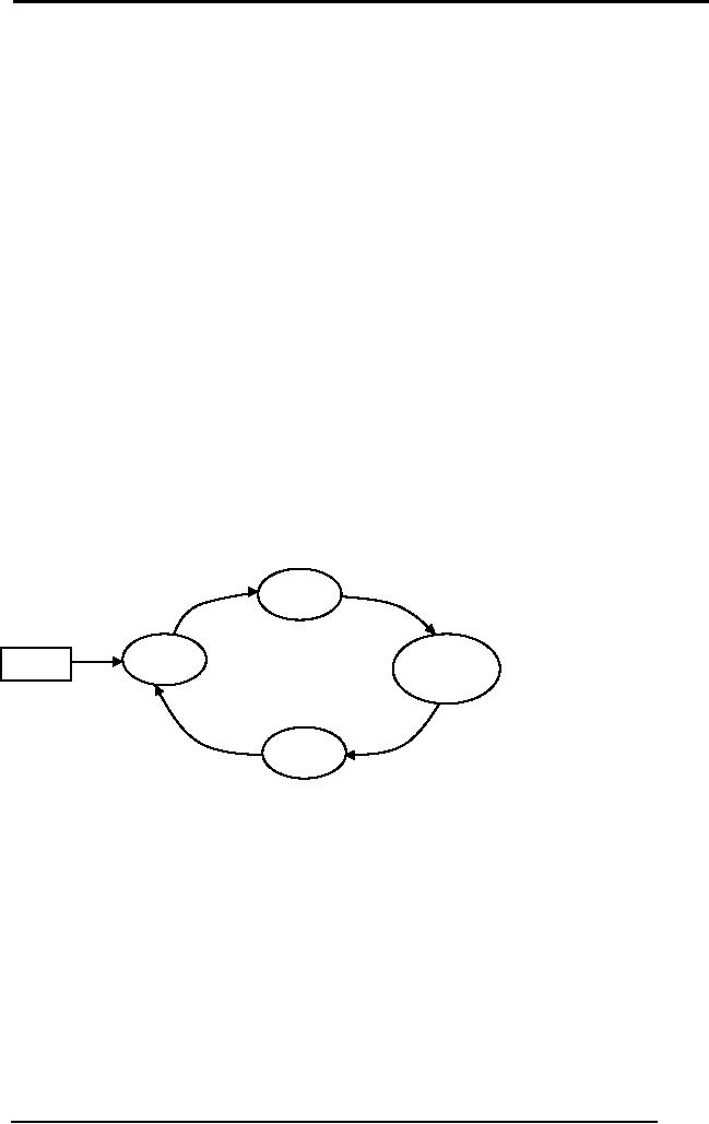
Artificial
Intelligence (CS607)
These
large feature spaces make
algorithms run slower. They
also
·
make
the training process longer.
The solution lies in finding
a
smaller
feature space which is the
subset of existing
features.
Feature
Space should show
discrimination between classes of
the
·
data.
Patient's height is not a
useful feature for
classifying whether
he is sick or
healthy
Training
·
· Training is
either supervised or
unsupervised.
· Remember
when we said:
· We assume
that the concept lies in
the hypothesis space.
So
we search
for a
hypothesis belonging to this
hypothesis
space
that best fits the
training examples, such that
the
output
given by the hypothesis is
same as the true output
of
concept
· Finding
the right hypothesis is the
goal of the training
session. So
neural networks are
doing function
approximation, and
training stops when it has
found the
closest
possible function that gives
the minimum error on
all
the
instances
· Training is
the heart of learning, in
which finding the
best
hypothesis
that covers most of the
examples is the
objective.
Learning is
simply done through
adjusting the weights of
the
network
Activation
function
Weighted
Similarity
Input
Sum
measure
of
input
Weight
updation
Similarity
Measurement
·
· A measure to
tell the difference between
the actual output of
the
network while training and
the desired labeled
output
· The
most common technique for
measuring the total error
in
each
iteration of the neural
network (epoch) is Mean
Squared
Error (MSE).
Validation
·
· During
training, training data is
divided into k data sets;
k-1
sets
are used for training,
and the remaining data
set is used
for
cross validation. This
ensures better results, and
avoids
over-fitting.
189

Artificial
Intelligence (CS607)
Stopping
Criteria
·
· Done
through MSE. We define a low
threshold usually
0.01,
which if
reached stops the training
data.
· Another
stopping criterion is the
number of epochs,
which
defines
how many maximum times
the data can be
presented to
the network for
learning.
Application
Testing
·
· A network is
said to generalize well when
the input-output
relationship
computed by the network is
correct (or nearly
so)
for
input-output pattern (test
data) never used in creating
and
training
the network.
7.21
Supervised
Given a
set of example input/output
pairs, find a rule that
does a good job of
predicting
the output associated with a
new input.
7.21.1
Back propagation
algorithm
1. Randomize
the weights {ws} to small
random values (both positive
and
negative)
2. Select a
training instance t,
i.e.,
a. the
vector {xk(t)}, i = 1,...,Ninp (a
pair of input and output
patterns),
from
the training set
3. Apply
the network input vector to
network input
4. Calculate
the network output vector
{zk(t)}, k = 1,...,Nout
5. Calculate
the errors for each of
the outputs k , k=1,...,Nout,
the difference
between
the desired output and
the network output
6. Calculate
the necessary updates for
weights -ws in a way that
minimizes
this
error
7. Adjust
the weights of the network
by - ws
8. Repeat
steps for each instance
(pair of inputoutput vectors) in
the training
set
until the error for
the entire system
7.22
Unsupervised
Given a
set of examples with no
labeling, group them into
sets called
·
clusters
A cluster
represents some specific
underlying patterns in the
data
·
Useful
for finding patterns in
large data sets
·
Form
clusters of input
data
·
Map the
clusters into outputs
·
Given a new
example, find its cluster,
and generate the associated
output
·
7.22.1
Self-organizing
neural networks: clustering, quantization,
function approximation, Kohonen
maps
1. Each
node's weights are
initialized
190

Artificial
Intelligence (CS607)
2. A data
input from training data
(vector) is chosen at random
and presented
to the
cluster lattice
3. Every
cluster centre is examined to
calculate which weights are
most like
the
input vector. The winning
node is commonly known as
the Best
Matching
Unit (BMU)
4. The
radius of the neighborhood of
the BMU is now calculated. Any
nodes
found
within this radius are
deemed to be inside the
BMU's neighborhood
5. Each
neighboring node's (the
nodes found in step 4)
weights are adjusted
to make
them more like the
input vector. The closer a
node is to the BMU,
the
more its weights get
altered
6. Repeat
steps for N
iterations
191

Artificial
Intelligence (CS607)
7.23
Exercise
1) We will
change the problem size
for SICK a little bit. If T
can take on 4
values,
and BP can take 5 values.
For conjunctive bias,
determine the
size of
instance space and hypothesis
space.
2) Is the
following concept possible
through conjunctive or
disjunctive
hypothesis? ( T
AND BP ) or ( T OR BP )
BP
H100
N010
L 001
LNH T
Appendix
MATLAB CODE
makeTrainData.m
trainData =
zeros(21, 100);
tempImage =
zeros(10,10);
for i =
1:7
filename =
strcat('alif', int2str(i),'.bmp');
tempImage =
imread(filename);
trainData(i,:) =
reshape(tempImage,1,100);
end
for i =
1:7
filename =
strcat('bay', int2str(i),'.bmp');
tempImage =
imread(filename);
trainData(i+7,:) =
reshape(tempImage,1,100);
end
for i =
1:7
filename =
strcat('jeem', int2str(i),'.bmp');
tempImage =
imread(filename);
trainData(i+14,:)
= reshape(tempImage,1,100);
end
targetData =
zeros(21,3);
targetData(1:7,1)
= 1;
targetData(8:14,2)
= 1;
targetData(15:21,3)
= 1;
192

Artificial
Intelligence (CS607)
save
'trainData' trainData targetData
;
makeTestData.m
testData =
zeros(9, 100);
tempImage =
zeros(10,10);
for i =
1:3
filename =
strcat('alif', int2str(i),'.bmp');
tempImage =
imread(filename);
testData(i,:) =
reshape(tempImage,1,100);
end
for i =
1:3
filename =
strcat('bay', int2str(i),'.bmp');
tempImage =
imread(filename);
testData(i+3,:) =
reshape(tempImage,1,100);
end
for i =
1:3
filename =
strcat('jeem', int2str(i),'.bmp');
tempImage =
imread(filename);
testData(i+6,:) =
reshape(tempImage,1,100);
end
targetData =
zeros(9,3);
targetData(1:3,1)
= 1;
targetData(4:6,2)
= 1;
targetData(7:9,3)
= 1;
save
'testData' testData
targetData;
193

Artificial
Intelligence (CS607)
trainNN.m
load
'trainData.mat';
minMax =
[min(trainData) ;
max(trainData)]';
bpn =
newff(minMax, [10 3],{'tansig'
'tansig'});
bpn.trainParam.epochs
= 15;
bpn.trainParam.goal
= 0.01;
bpn =
train(bpn,trainData',targetData');
save
'bpnNet' bpn;
testNN.m
load('trainData');
load('bpnNet');
Y = sim(bpn,
trainData');
[X,I] =
max(Y);
errorCount =
0;
for i = 1 :
length(targetData)
if ceil(i/7) ~=
I(i)
errorCount =
errorCount + 1;
end
end
percentageAccuracyOnTraining
= (1-(errorCount/length(targetData))) *
100
%%%%%%%%%%%%%%%%%%%%%%%%%%
load('testData');
Y = sim(bpn,
testData');
[X,I] =
max(Y);
errorCount =
0;
for i = 1 :
length(targetData)
if ceil(i/3) ~=
I(i)
errorCount =
errorCount + 1;
end
end
percentageAccuracyOnTesting
= (1-(errorCount/length(targetData))) *
100
194