 |
ECONOMIC GROWTH:THE SOLOW MODEL, Saving and investment |
| << ISSUES IN UNEMPLOYMENT:Public Policy and Job Search |
| ECONOMIC GROWTH (Continued ):The Steady State >> |

Macroeconomics
ECO 403
VU
LESSON
19
ECONOMIC
GROWTH
Issues in
Economic Growth
·
Learn
the closed economy Solow
model
·
See
how a country's standard of
living depends on its saving
and population growth
rates
·
Learn
how to use the "Golden
Rule"
to
find the optimal savings
rate and capital
stock
Per
Capita Income of Selected
Countries, 2004 (in US
$)
Norway
43,350
Saudi
Arabia
8,530
Switzerland
39,880
Mexico
6,230
United
States
37,610
Malaysia
3,780
Japan
34,510
Brazil
2,710
United
Kingdom
28,350
Russia
2,610
Belgium
25,820
Egypt
1,390
Germany
25,250
China
1,100
France
24,770
Indonesia
810
Australia
21,650
India
530
Italy
21,560
Pakistan
470
Kuwait
16,340
Bangladesh
400
Korea
12,020
Nigeria
320
THE
SOLOW MODEL
·
Due to
Robert Solow, won Nobel
Prize for contributions to
the study of economic
growth
·
A
major paradigm:
Widely
used in policy making
Benchmark
against which most
recent
growth theories are
compared
·
Looks at
the determinants of economic
growth and the standard of
living in the long
run
·
The
Solow
Growth Model is designed to
show how growth in the
capital stock, growth
in
the labor force, and
advances in technology interact in an
economy, and how
they
affect
a nation's total output of
goods and services.
70
Macroeconomics
ECO 403
VU
How
Solow model is
different
1.
K
is no longer fixed: investment
causes it to grow, depreciation
causes it to shrink.
2.
L
is no longer fixed: population
growth causes it to
grow.
3.
The
consumption function is
simpler.
4.
No
G
or
T
(only
to simplify presentation; we can
still do fiscal policy
experiments)
5.
Cosmetic
differences.
The
production function
Let's
analyze the supply and
demand for goods, and
see how much output is
produced at any
given
time and how this
output is allocated among
alternative uses.
The
production function represents
the transformation of inputs
(labor
(L), capital (K),
and
production technology) into
outputs
(final
goods and services for a
certain time period).
·
In
aggregate terms: Y
=
F (K,
L )
·
Define:
y =
Y/L
=
output per worker
k
=
K/L
=
capital per worker
·
Assume
constant returns to
scale:
zY
=
F (zK,
zL )
for any z
>
0
·
Pick
z =
1/L.
Then
Y/L
=
F (K/L
,
1)
y
=
F (k,
1)
y
=
f(k)
where
f(k)
=
F (k,
1)
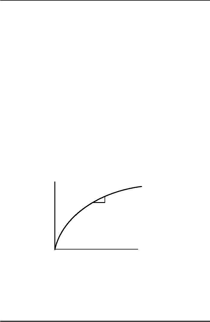
Output
per
worker,
y
f(k)
MPK
=f(k
+1)
f(k)
1
Note:
this production
function
exhibits
diminishing
MPK.
Capital
per
worker,
k
The
national income
identity
·
Y=C+I
(remember,
no G
)
71
Macroeconomics
ECO 403
VU
In
"per worker" terms:
·
y=c+i
where
c = C/L
and i = I/L
The
consumption function
·
s =
the saving rate, the
fraction of income that is
saved (s is an exogenous
parameter)
·
Note: s is
the only lowercase variable
that is not equal to its
uppercase version
divided
by L
·
Consumption
function: c = (1s)y (per
worker)
Saving
and investment
·
saving
(per worker) = sy
·
National
income identity is y = c
+
i
Rearrange
to get: i = y c = sy
(investment
= saving)
·
Using
the results above,
i
= sy = sf(k)
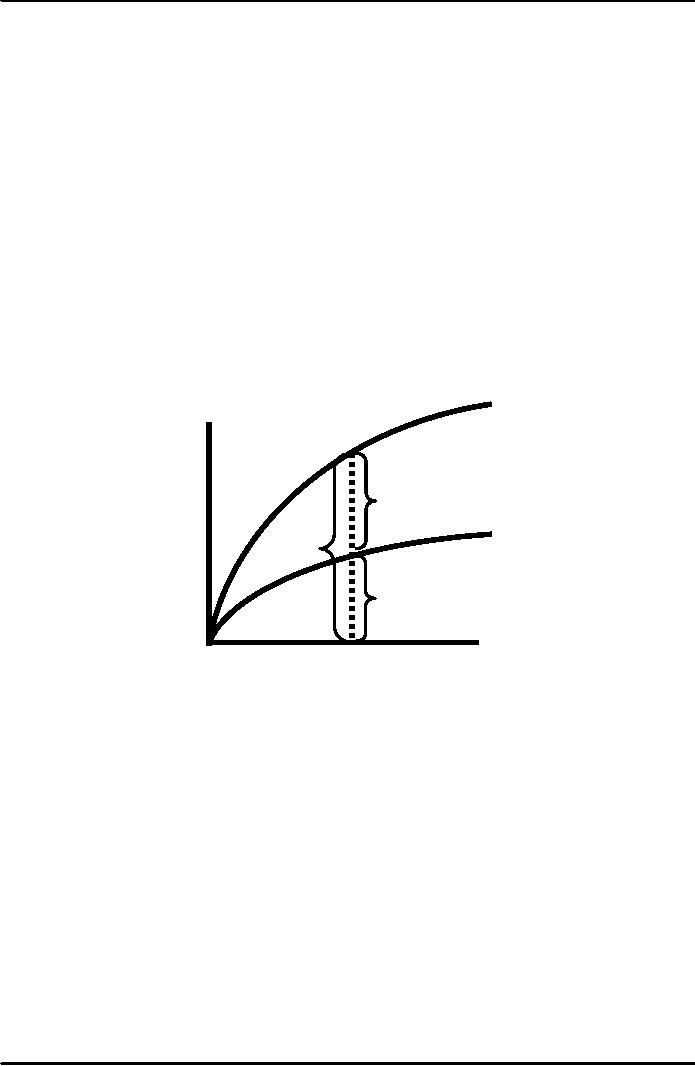
Output,
consumption, and
investment
Output
per
f(k)
worker,
y
c1
sf(k)
y1
i1
Capital
per
k1
worker,
k
72

Macroeconomics
ECO 403
VU
Depreciation
Depreciation
per
δ
=
the rate of
depreciation
worker,
δk
=
the fraction of the capital
stock that
wears
out each period
δk
δ
1
Capital
per
worker,
k
Capital
accumulation
The
basic idea:
Investment
makes the capital stock
bigger, depreciation makes it
smaller.
Change
in capital stock= investment
depreciation
Δk =
δk
i
Since
i = sf (k), this
becomes:
Δk =
s f(k) δk
The
equation of motion for
k
Δk =
s f(k) δk
·
the
Solow model's central
equation
·
Determines
behavior of capital over
time which, in turn,
determines behavior of all
of
the
other endogenous
variables
because
they all depend on k.
e.g., income per
person:
y
=
f(k)
Consumption
.per person:
c
=
(1s)
f(k)
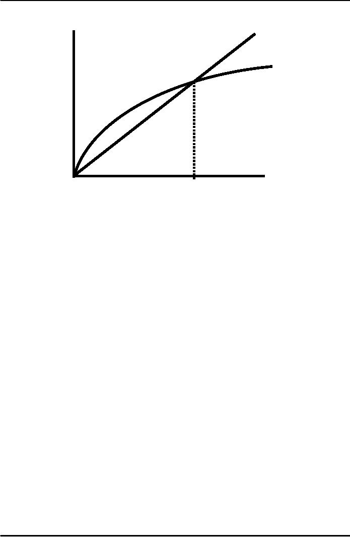
The
steady state
If
investment is just enough to
cover depreciation
[sf(k)
=
δk
],
then
capital per worker will
remain constant:
Δk
=
0.
This
constant value, denoted
k*,
is called the steady state
capital stock.
73
Macroeconomics
ECO 403
VU
Investment
and
depreciation
δk
sf(k)
k*
Capital
per
worker,
k
74
Table of Contents:
- INTRODUCTION:COURSE DESCRIPTION, TEN PRINCIPLES OF ECONOMICS
- PRINCIPLE OF MACROECONOMICS:People Face Tradeoffs
- IMPORTANCE OF MACROECONOMICS:Interest rates and rental payments
- THE DATA OF MACROECONOMICS:Rules for computing GDP
- THE DATA OF MACROECONOMICS (Continued ):Components of Expenditures
- THE DATA OF MACROECONOMICS (Continued ):How to construct the CPI
- NATIONAL INCOME: WHERE IT COMES FROM AND WHERE IT GOES
- NATIONAL INCOME: WHERE IT COMES FROM AND WHERE IT GOES (Continued )
- NATIONAL INCOME: WHERE IT COMES FROM AND WHERE IT GOES (Continued )
- NATIONAL INCOME: WHERE IT COMES FROM AND WHERE IT GOES (Continued )
- MONEY AND INFLATION:The Quantity Equation, Inflation and interest rates
- MONEY AND INFLATION (Continued ):Money demand and the nominal interest rate
- MONEY AND INFLATION (Continued ):Costs of expected inflation:
- MONEY AND INFLATION (Continued ):The Classical Dichotomy
- OPEN ECONOMY:Three experiments, The nominal exchange rate
- OPEN ECONOMY (Continued ):The Determinants of the Nominal Exchange Rate
- OPEN ECONOMY (Continued ):A first model of the natural rate
- ISSUES IN UNEMPLOYMENT:Public Policy and Job Search
- ECONOMIC GROWTH:THE SOLOW MODEL, Saving and investment
- ECONOMIC GROWTH (Continued ):The Steady State
- ECONOMIC GROWTH (Continued ):The Golden Rule Capital Stock
- ECONOMIC GROWTH (Continued ):The Golden Rule, Policies to promote growth
- ECONOMIC GROWTH (Continued ):Possible problems with industrial policy
- AGGREGATE DEMAND AND AGGREGATE SUPPLY:When prices are sticky
- AGGREGATE DEMAND AND AGGREGATE SUPPLY (Continued ):
- AGGREGATE DEMAND AND AGGREGATE SUPPLY (Continued ):
- AGGREGATE DEMAND AND AGGREGATE SUPPLY (Continued )
- AGGREGATE DEMAND AND AGGREGATE SUPPLY (Continued )
- AGGREGATE DEMAND AND AGGREGATE SUPPLY (Continued )
- AGGREGATE DEMAND IN THE OPEN ECONOMY:Lessons about fiscal policy
- AGGREGATE DEMAND IN THE OPEN ECONOMY(Continued ):Fixed exchange rates
- AGGREGATE DEMAND IN THE OPEN ECONOMY (Continued ):Why income might not rise
- AGGREGATE SUPPLY:The sticky-price model
- AGGREGATE SUPPLY (Continued ):Deriving the Phillips Curve from SRAS
- GOVERNMENT DEBT:Permanent Debt, Floating Debt, Unfunded Debts
- GOVERNMENT DEBT (Continued ):Starting with too little capital,
- CONSUMPTION:Secular Stagnation and Simon Kuznets
- CONSUMPTION (Continued ):Consumer Preferences, Constraints on Borrowings
- CONSUMPTION (Continued ):The Life-cycle Consumption Function
- INVESTMENT:The Rental Price of Capital, The Cost of Capital
- INVESTMENT (Continued ):The Determinants of Investment
- INVESTMENT (Continued ):Financing Constraints, Residential Investment
- INVESTMENT (Continued ):Inventories and the Real Interest Rate
- MONEY:Money Supply, Fractional Reserve Banking,
- MONEY (Continued ):Three Instruments of Money Supply, Money Demand