Digital Image Definitions:COMMON VALUES, Types of operations, VIDEO PARAMETERS

<< Introduction

Tools:CONVOLUTION, FOURIER TRANSFORMS, Circularly symmetric signals >>

...Image Processing Fundamentals

regionsofinterest, ROIs, or simply regions. This concept reflects the fact that

images frequently contain collections of objects each of which can be the basis for a

region. In a sophisticated image processing system it should be possible to apply

specific image processing operations to selected regions. Thus one part of an image

(region) might be processed to suppress motion blur while another part might be

processed to improve color rendition.

The amplitudes of a given image will almost always be either real numbers or

integer numbers. The latter is usually a result of a quantization process that converts

a continuous range (say, between 0 and 100%) to a discrete number of levels. In

certain image-forming processes, however, the signal may involve photon counting

which implies that the amplitude would be inherently quantized. In other image

forming procedures, such as magnetic resonance imaging, the direct physical

measurement yields a complex number in the form of a real magnitude and a real

phase. For the remainder of this book we will consider amplitudes as reals or

integers unless otherwise indicated.

Digital Image Definitions

A digital image a[m,n] described in a 2D discrete space is derived from an analog

image a(x,y) in a 2D continuous space through a sampling process that is

frequently referred to as digitization. The mathematics of that sampling process will

be described in Section 5. For now we will look at some basic definitions

associated with the digital image. The effect of digitization is shown in Figure 1.

The 2D continuous image a(x,y) is divided into N rows and M columns. The

intersection of a row and a column is termed a pixel. The value assigned to the

integer coordinates [m,n] with {m=0,1,2,...,M1} and {n=0,1,2,...,N1} is a[m,n].

In fact, in most cases a(x,y)--which we might consider to be the physical signal

that impinges on the face of a 2D sensor--is actually a function of many variables

including depth (z), color (λ), and time (t). Unless otherwise stated, we will

consider the case of 2D, monochromatic, static images in this chapter.

...Image Processing Fundamentals

Columns

Value = a(x, y, z, λ, t)

Figure 1: Digitization of a continuous image. The pixel at coordinates

[m=10, n=3] has the integer brightness value 110.

The image shown in Figure 1 has been divided into N = 16 rows and M = 16

columns. The value assigned to every pixel is the average brightness in the pixel

rounded to the nearest integer value. The process of representing the amplitude of

the 2D signal at a given coordinate as an integer value with L different gray levels is

usually referred to as amplitude quantization or simply quantization.

2.1 COMMON VALUES

There are standard values for the various parameters encountered in digital image

processing. These values can be caused by video standards, by algorithmic

requirements, or by the desire to keep digital circuitry simple. Table 1 gives some

commonly encountered values.

Parameter

Symbol

Typical values

Rows

256,512,525,625,1024,1035

Columns

256,512,768,1024,1320

Gray Levels

2,64,256,1024,4096,16384

Table 1: Common values of digital image parameters

Quite frequently we see cases of M=N=2K where {K = 8,9,10}. This can be

motivated by digital circuitry or by the use of certain algorithms such as the (fast)

Fourier transform (see Section 3.3).

...Image Processing Fundamentals

The number of distinct gray levels is usually a power of 2, that is, L=2B where B is

the number of bits in the binary representation of the brightness levels. When B >1

we speak of a gray-level image; when B =1 we speak of a binary image. In a binary

image there are just two gray levels which can be referred to, for example, as

"black" and "white" or "0" and "1".

2.2 CHARACTERISTICS OF IMAGE OPERATIONS

There is a variety of ways to classify and characterize image operations. The reason

for doing so is to understand what type of results we might expect to achieve with a

given type of operation or what might be the computational burden associated with

a given operation.

2.2.1 Types of operations

The types of operations that can be applied to digital images to transform an input

image a[m,n] into an output image b[m,n] (or another representation) can be

classified into three categories as shown in Table 2.

Operation

Characterization

Generic

Complexity/Pixel

· Point

constant

the output value at a specific coordinate is dependent

only on the input value at that same coordinate.

· Local

the output value at a specific coordinate is dependent on

the input values in the neighborhood of that same

coordinate.

· Global

the output value at a specific coordinate is dependent on

all the values in the input image.

Table 2: Types of image operations. Image size = N × N; neighborhood size

= P × P . Note that the complexity is specified in operations per pixel.

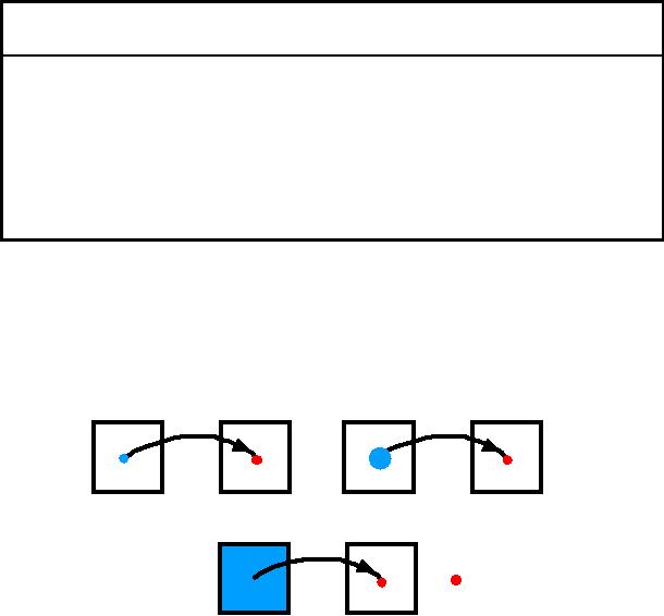
This is shown graphically in Figure 2.

Point

Local

Global

= [m=mo, n=no]

Figure 2: Illustration of various types of image operations

...Image Processing Fundamentals

2.2.2 Types of neighborhoods

Neighborhood operations play a key role in modern digital image processing. It is

therefore important to understand how images can be sampled and how that relates

to the various neighborhoods that can be used to process an image.

· Rectangular sampling In most cases, images are sampled by laying a

rectangular grid over an image as illustrated in Figure 1. This results in the type of

sampling shown in Figure 3ab.

· Hexagonal sampling An alternative sampling scheme is shown in Figure 3c and

is termed hexagonal sampling.

Both sampling schemes have been studied extensively [1] and both represent a

possible periodic tiling of the continuous image space. We will restrict our

attention, however, to only rectangular sampling as it remains, due to hardware and

software considerations, the method of choice.

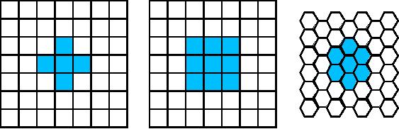
Local operations produce an output pixel value b[m=mo,n=no] based upon the pixel

values in the neighborhood of a[m=mo,n=no]. Some of the most common

neighborhoods are the 4-connected neighborhood and the 8-connected

neighborhood in the case of rectangular sampling and the 6-connected

neighborhood in the case of hexagonal sampling illustrated in Figure 3.

Figure 3a

Figure 3b

Figure 3c

Rectangular sampling

Hexagonal sampling

4-connected

8-connected

6-connected

2.3 VIDEO P ARAMETERS

We do not propose to describe the processing of dynamically changing images in

this introduction. It is appropriate--given that many static images are derived from

video cameras and frame grabbers-- to mention the standards that are associated

with the three standard video schemes that are currently in worldwide use NTSC,

PAL, and SECAM. This information is summarized in Table 3.

Table of Contents: